Download
1 / 73
750 likes | 784 Vues
Discover how beam parameters influence image clarity in the Scanning Electron Microscope (SEM) technology. Explore components like filaments, lenses, electron scattering, and image formation. Learn about field of view, resolution down to 1 nm, and beam accelerator technologies.

E N D
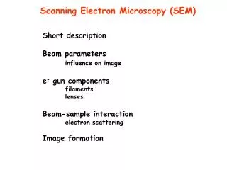
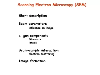
Scanning Electron Microscopy (SEM) Short description Beam parameters influence on image e- gun components filaments lenses Beam-sample interaction electron scattering Image formation
Scanning Electron Microscope (SEM) Field of view: 5x 5 mm2 – 500 x 500 nm2 V-shaped Filament Extractor Resolution: down to 1 nm Beam accelerator Deflecting Plates Electron Column Image Display Primary e- Beam Scan quadrupole e- Detector Backscattered Electrons Sample
Optical axis S How to sweep an electron beam First coil deviate beam from optical axis Second coil brings beam back at optical axis on the pivot point Image formation point by point collecting signal at each raster point L L = raster length on sample W = working distance S = raster length on screen Magnification = S/L L = 10 m, S = 10 cm M depends on working distance
Effect of beam parameters on image V0 = beam voltage ip = beam current p = beam convergence angle dp = beam diameter at sample
Effect of beam parameters on image Resolution High resolution mode Noise on signal ip = beam current dp = beam diameter Good compromise ip = 1 pA, dp = 15 nm ip = 320 pA, dp = 130 nm ip = 5 pA, dp = 20 nm High current mode Resolution too low
Effect of beam parameters on image Depth of focus If p is small, dp changes little with depth, so features at different heights can be in focus p = 15 mrad p = 1 mrad
Effect of beam parameters on image Electron energy V0 < 5 kV, beam interaction limited to region close to surface, info on surface details V0 15 - 30 kV, beam penetrates into sample, info on interior of sample V0 = beam voltage
Electron column e- are produced and accelerated Beam is reduced to increase resolution Beam is focused on sample
Filament Wehnelt: focuses e- inside the gun Controls intensity of emitted e- Grid connected to filament with variable resistor e- exit filament following + lines The equipontential line shape has focussing effect and determines 0 and d0 e- are accelerated to anode and the hole allows a fraction of this e- to reach the lenses
Filament Equipotential lines Filament head Electron beam The equipontential line shape has focussing effect and determines 0 and d0 Electron column
Filament types Lanthanum hexaboride (LaB6) Tungsten hairpin (most common) 0.120 mm Tungsten wire Operating principle: thermionic electron emission LaB6 crystal 0.20 mm
Filament types thermionic electron emission Ac = 120 A/cm2K2 Ew = work function To reduce filament evaporation operate the electron gun at the lowest possible temperature Materials of low work function are desired. Tungsten hairpin Lanthanum hexaboride (LaB6) Ew = 4.5 eV Jc = 3.4 A/cm2 at 2700 K Lifetime 50-150 hours Energy width 0.7 eV Operating pressure 10-5 mbar Ew = 2.5 eV Jc = 40 A/cm2 at 1800 °K Lifetime 200-1000 hours Energy width 0.3 eV Operating pressure 10-6 mbar
Filament types Thermal Field Emission Operating principle: thermionic electron emission + Tunnelling W-Zr crystal 0.20 mm I = 1 104 A/cm2 at 1800 °C Lifetime > 1000 hours Energy width 0.1 eV Small source dimension (few nm) Operating pressure 10-9 mbar
dp R p E gun brightness Beam current changes throughout the column Brightness is conserved throughout the column Tungsten hairpin Lanthanum hexaboride (LaB6) Thermal Field Emission dp: 30 – 100 m dp: 5 – 50 m dp: 5 nm = 106 A/sr cm2 = 108 A/sr cm2 = 105 A/sr cm2
Electromagnetic Lenses Demagnification of beam crossover image (d0) to get high resolution (small dp) d0: 5 – 100 m for filaments d0: 5 nm for TFE High demag needed Low demag needed Beam focussing Fringe field coils radial parallel
Electromagnetic Lenses Focusing process e- interacts withBr and Bzseparately -e (vz x Br) produces a force into screen Fqin giving e- rotational velocity vqin vqin interacts with Bz produces a force toward optical axis Fr =-e (vqin x Bz) f = focal length the distance from the point where an electron first begins to change direction to the point where it crosses the axis. The actual trajectory of the electron will be a spiral The final image shows this spiraling action as a rotation of the image as the objective lens strength is changed.
Electromagnetic Lenses Lens coil current and focal length I = lens coil current N = number of coils V0 = accelerating voltage Increasing the strength (current) of the lens reduces the focal distance
Comparison to optical lenses Demagnification of beam crossover image (d0) = object Beam crossover d0 = tungsten diameter = 50 m Scaling from the figure, the demag factor is 3.4 so d1 = d0/m = 14.7 m CONDENSER LENSES: the aim is to reduce the beam diameter
Objective Lenses They should contain: Scanning coil Stigmator Beam limiting aperture Scope: focus beam on sample They also provide further demagnification Pinhole No B outside Large samples Long working distances (40 mm) High aberrations Snorkel B outside lens Large samples Separation of secondary from backscattered e- Long working distances Low aberrations Immersion Sample in B field Small samples Short working distances (3 mm) Highest resolution Low aberrations Separation of secondary from backscattered e-
Effect of aperture size Aperture size: 50 – 500 m Decrease 1 for e- entering OL to a a determines the depth of focus Determines the beam current Reduces aberrations
Effect of working distance Increase in WD increase in q m smaller larger d lower resolution but longer depth of focus
Effect of condenser lens strenght Strong Weak Decrease q1 and increase p2 larger m Higher Ibeam Lower Ibeam Lower dp Higher dp Increase in condenser strenght (current) longer q larger m and smaller d Also it brings a beam current reduction, so a compromise between current and resolution is needed
Gaussian probe diameter The distribution of emission intensity from filament is gaussian with size dG dG = FWHM With no aberrations, keeping dG constant would allow to increase ip by only increasing p
Spherical aberrations Origin: e- far from optical axis are deflected more strongly e- along PA gives rise to gaussian image plane No aberration e- along PB cross the optical axis in ds So at the focal plane there is a disk and not a point Spherical aberration disk of least confusion For immersion and snorkel Cs ~ 3 mm For pinholes Cs ~ 20-30 mm Cs = Spherical aberration coefficient f So one need to put an aperture
Aperture diffraction To estimate the contribution to beam diameter one takes half the diameter of the diffraction disk nm sr eV
Chromatic aberrations Origin: initial energy difference of accelerated electrons Chromatic aberration disk of least confusion For tungsten filament E = 3 eV At 30 KeV E/E0 = 10-4 At 3 KeV E/E0 = 10-3 Cs = Chromatic aberration coefficient f
Astigmatism Origin: machining errors, asymmetry in coils, dirt Result: formation ow two differecnt focal points Effect on image: Stretching of points into lines Can be compensated with octupole stigmator
Beam-sample interaction Simulation of e- trajectories Backscattered e- Silicon V0 = 20 KV TFE, = 1 108 A/sr cm2 dp = 1 nm Ib = 60 pA Main reason of large interaction volume: Elastic Scattering Inelastic scattering
Beam-sample interaction 0 Elastic Scattering Elastic scattering cross section Z = atomic number; E = e- energy (keV); A = atomic number N0 = Avogadro’s number; = atomic density Elastic mean free path = distance between scattering events Silicon = 2.33 g/cm3 Z = 14 A = 28 N0 = 6.022 1023
Beam-sample interaction Inelastic Scattering Inelastic scattering energy loss rate Z = atomic number A= atomic number N0 = Avogadro’s number = atomic density Ei = e- energy in any point inside sample J = average energy loss per event Eb = 20 KeV The path of a 20 KeV e- is of the order of microns, so the interaction volume is about few microns cube
Beam-sample interaction 20 KeV beam incident on PMMA with different time periods Interaction volume Simulation Energy transferred to sample
Influence of beam parameters on beam-sample interaction Beam energy 10 KeV 20 KeV Fe 30 KeV Elastic scattering cross section Inelastic scattering energy loss rate Longer Lower loss rate
Influence of beam parameters on beam-sample interaction Smaller and asymmetric interaction volume Incidence angle 45° Fe 60° surface surface Scattering of e- out of the sample Reduced depth Same lateral dimensions
Influence of sample on beam-sample interaction Atomic number V0 = 20 keV Fe (Z=26) C (Z=6) Fe, k shell C, k shell Elastic scattering cross section 10% to 50% of the beam electrons are backscattered They retain 60% to 80% of the initial energy of the beam Inelastic scattering energy loss rate Reduced linear dimensions of interaction volume
Influence of sample on beam-sample interaction Atomic number V0 = 20 keV Ag (Z=47) U (Z=92) U, k shell Ag, k shell More spherical shape of interaction volume
Signal from interaction volume (what do we see?) Backscattered electrons Secondary electrons Backscattered e-
BSE dependence Backscattered electron coefficient Monotonic increase Relationship between and a sample property (Z) This gives atomic number contrast 60° If different atomic species are present in the sample Ci = weight concentration
BSE dependence Incidence angle n = intensity at normal Line length: relative intensity of BSE Strong influence on BSE detector position 60°
BSE dependence Energy distribution Lateral spatial distribution The energy of each BSE depends on the trajectory inside sample, hence different energy losses Region good for high resolution Region I: E up to 50 % Becomes peaked with increasing Z Gives rise to loss in lateral resolution At low Z the external region increases
BSE dependence Sampling depth Percent of Fraction of maximum e- penetration (microns) RKO defines a circle on the surface (center in the beam) spanning the interaction volume Sampling depth is typically 100 -300 nm for beam energies above 10 keV
Signal from interaction volume (what do we see?) Energy distribution of electrons emitted by a solid Secondary electrons Energy: 5 – 50 eV Probability of e- escape from solid = e- mean free path
Secondary electrons Origin: electron elastic and inelastic scattering SURFACE SENSITIVE SE1 = secondary due directly to incident beam Beam resolution BSE resolution SE2 = secondary generated by backscattered electrons Low backscattering cross section Carbon: SE2 /SE1 = 0.18 Aluminum: SE2 /SE1 = 0.48 Copper: SE2 /SE1 = 0.9 High backscattering cross section Gold: SE2 /SE1 = 1.5 SE Intensity angular distribution: cos
Image formation Backscattered e- Secondary e- Volume sensitive Surface sensitive Sampling depth ~ 100 -300 nm
Image formation Many different signals can be extracted from beam-sample interaction So the information depends on the signal acquired, is not only topography
Image formation The beam is scanned along a single vector (line) and the same scan generator is used to drive the horizontal scan on a screen Signals to be recorded For each point the detector collects a current and the intensity is plotted or the intensity is associated with a grey scale at a single point A one to one correspondence is established between a single beam location and a single point of the display Magnification M = LCRT/Lsample But the best way is to calibrate the instrument
Image formation Digital image: array (x,y,Signal) 8 bits = 28 = 256 gray levels Signal: output of ADC Resolution = 2n 16 bits = 216 = 65536 gray levels Pixel = picture element Pixel is the size of the area on the sample from which information is collected Actually is a circle Considering the matrix defining the: Pixel edge dimension Length of the scan on sample number of steps along the scan line The image is focused when the signal come only from a the location where the beam is addressed At high magnification there will be overlap between two pixel
Image formation For a given experiment (sample type) and experimental conditions (beam size, energy) the limiting magnification should obtained by calculating the area generating signal taking into account beam-sample interactions and compare to pixel size beam Area producing BSe- V0 = 10 keV, dB = 50 nm on Al, dBSE = 1.3 m deff = 1.3 m on AudBSE = 0.13 m deff = 0.14 m 10x 10 cm display There is overlapping of pixel signal intensity Different operation settings for low and high magnification
Depth of field Depth of field D = distance along the lens axis (z) in the object plane in which an image can be focused without a loss of clarity. To calculate D, we need to know where from the focal plane the beam is broadened Broadening means adjacent pixel overlapping The vertical distance required to broaden a beam r0 to a radius r (causing defocusing) is For small angles
Depth of field How much is r? On a CRT defocusing is visible when two pixels are overlapped r = 1 pixel (on screen 0.1 mm) But 1 pixel size referred to sample depends on magnification To increase D, we can either reduce M or reduce beam divergence Beam divergence is defined by the beam defining aperture