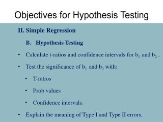
Objectives for Hypothesis Testing
Objectives for Hypothesis Testing. Simple Regression B. Hypothesis Testing Calculate t-ratios and confidence intervals for b 1 and b 2 . Test the significance of b 1 and b 2 with: T-ratios Prob values Confidence intervals. Explain the meaning of Type I and Type II errors.

Objectives for Hypothesis Testing
E N D
Presentation Transcript
Objectives for Hypothesis Testing • Simple Regression B. Hypothesis Testing • Calculate t-ratios and confidence intervals for b1 and b2 . • Test the significance of b1 and b2 with: • T-ratios • Prob values • Confidence intervals. • Explain the meaning of Type I and Type II errors.
The Model for Hypothesis Testing The Simple Linear Regression Model
Hypothesis Testing Goal: Does X significantly affect Y? Is β2 = 0 ? Conduct a hypothesis test of the form: H0: β2 = 0 Null hypothesis (X does not affect Y) H1: β2 ≠ 0 Alternative hypothesis (X affects Y) Use a test statistic, the t-ratio, given by: t = b2/[se(b2)] where se(b2) = the standard error of b2 .
The t-distribution • Under the null hypothesis, β2 = 0, the t-ratio is distributed according to the t-distribution, i.e., t = b2/[se(b2)] ~ t (N-2) • If the null hypothesis is not true, the t-ratio does not have a t-distribution. • The t-distribution is a bell-shaped curve. • It looks like the normal distribution, except it is more spread out, with a larger variance and thicker tails. • The t-distribution converges to a normal distribution as the sample size gets large (as N ). • The shape of the t-distribution is controlled by a single parameter called the degrees of freedom, often abbreviated as df, where df = N – k , N = number of observations and k = number of parameters.
Statistics Trivia The t-distribution was developed by William Sealy Gosset, a brewing chemist at the Guinness brewery in Ireland. He developed the t-test to ensure consistent quality from each batch of Guinness beer. Guinness allowed Gosset to publish his results, but only under the condition that the data remain confidential and that he publish under a different name. Gosset published under the pseudonym “Student” and the distribution became known as the Student t-distribution.
The t-distribution Figure 3.1 Critical Values from a t-distribution
Two-tail Tests with Alternative “Not Equal To” (≠) Figure 3.4 The rejection region for a two-tail test of H0: βk = c against H1: βk ≠ c
Tests of Significance • Model: Rent = β1 + β2 Distance + e Assume all other assumptions of the simple regression model are met. 2. The null hypothesis is : H0: β2 = 0 The alternative hypothesis is: H1: β2 ≠ 0 . 3. The test statistic is: t = b2/[se(b2)] ~ t (N-2) if the null hypothesis is true. • Let us select α = .05. Note N = 32. What are the degrees of freedom and critical values? df = 30; t = 2.042 What is the rejection region? t - 2.042; t 2.042; if - 2.042 < t < 2.042, we do not reject the null hypothesis
Regression of Rent on Distance • Calculate the t-ratio on the distance parameter. • Test for the significance of the distance parameter on rent using a t-test. The REG Procedure Model: MODEL1 Dependent Variable: rent Number of Observations Read 32 Parameter Estimates Parameter Standard Variable DF Estimate Error t Value Pr > |t| Intercept 1 486.18871 59.78625 8.13 <.0001 distance 1 -2.57625 3.16619 0.4222
Significance of the Distance Parameter in the Rent Equation • What is the value of the t-ratio on b 2? t = -2.58/3.17 = - 0.81 • What do you conclude? • Since t > -2.042 and t < 2.042, we do not reject the null hypothesis. • The parameter estimate on distance, b2, is not significantly different from zero. • Distance is not a significant determinant of rent.
The p-Value Graphically, the P-value is the area in the tails of the distribution beyond |t|. That is, if t is the calculated value of the t-statistic, and if H1: βK ≠ 0, then: p = sum of probabilities to the right of |t| and to the left of – |t| According to the p-value on the parameter on distance in the rent equation, do you reject the null hypothesis?
Regression of Rent on Distance The REG Procedure Model: MODEL1 Dependent Variable: rent Number of Observations Read 32 Number of Observations Used 32 Parameter Estimates Parameter Standard Variable DF Estimate Error t Value Pr > |t| Intercept 1 486.18871 59.78625 8.13 <.0001 distance 1 -2.57625 3.16619 -0.81 0.4222
Regression of Coffee on Age for Coffee Drinkers For the following regression estimates, test the hypothesis that the parameter estimate on age is significantly different from zero using a t-test and a p-value test. The REG Procedure Model: MODEL1 Dependent Variable: coffee Number of Observations Read 13 Parameter Estimates Parameter Standard Variable DF Estimate Error t Value Pr > |t| Intercept 1 65.53119 16.73502 3.92 0.0024 age 1 -1.36918 0.58207 -2.35 0.0383
Test of Significance of Age in Coffee Regression for Sample of Coffee Drinkers α= .05. N = 13 df = 13-2 = 11. t = 2.201 Since t = -2.35 < -2.201 we reject the null hypothesis and conclude that age significantly affects coffee consumption for coffee drinkers. The p-value = 0.0383 < .05 also indicates we should reject H0.