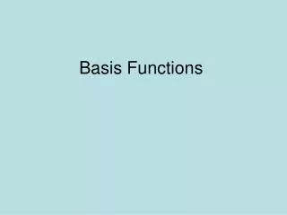
Basis Functions
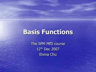
Basis Functions. v = 4 i + 2 j. j. i. What’s a basis ?. Can be used to describe any point in space. e.g. the common Euclidian basis (x, y, z) forms a basis according to which you can describe a point by its coordinate on each axis. y. 2. i. 4. x.


Basis Functions
E N D
Presentation Transcript
v = 4 i + 2 j j i What’s a basis ? Can be used to describe any point in space. e.g. the common Euclidian basis (x, y, z) forms a basis according to which you can describe a point by its coordinate on each axis. y 2 i 4 x More precisely, the vector going from the origin to that point is equal to a weighted sum of the units vectors of the axes.
Basis functions In fMRI instead of describing a point you want to describe a curve or function (% signal change in function of time) by decomposing it in simpler functions. If you use only one function you have a limited power to describe the % signal change variations, so it’s better to use a number of functions, which constitutes a set of basis functions. That’s why SPM offers different sets of basis functions to model the % signal change variations. f(t) h1(t) h2(t) h3(t) Fourier analysis: the complex wave at the top can be decomposed into the sum of the three simpler waves shown below. f(t)=h1(t)+h2(t)+h3(t)
Basis functions offered by SPM The most general are the finite impulse response (A) and Fourier (B) basis sets, which make minimal assumptions about the shape of the response. Finite Impulse Response (FIR) Fourier Linear combination of the basis functions can capture any shape of response up to a specified timescale.
More parsimonious basis sets make various assumptions about the shape of the HRF. Gamma function One popular choice is the gamma function, which has been shown to provide a reasonably good fit to the impulse response, although it lacks an undershoot. The set used in SPM is more parsimonious in that fewer functions are required to capture the typical range of impulse responses than are required by the Fourier or FIR sets, reducing the degrees of freedom used in the design matrix and allowing more powerful statistical tests.
Canonical haemodynamic response function (HRF) Typical BOLD response to an impulse stimulation. The response peaks approximately 5 sec after stimulation, and is followed by an undershoot (at high magnetic files, an initial undershoot can sometimes be observed).
Neural signal convolved with a canonical HRF to produce the predicted BOLD signal.
Fits of a boxcar epoch model with (red) and without (black) convolution by a canonical HRF, together with the data.
Residuals after fits of models with and without HRF convolution. Large systematic errors for model without HRF convolution (black) at onset of each block.
Limits of HRF • - General shape of the BOLD impulse response similar across early sensory regions, such as V1 and S1. • Variability across higher cortical regions regions, presumably due mainly to variations in the vasculature of different regions. • Considerable variability across people. • These types of variability can be accommodated by expanding the HRF in terms of temporal basis functions.
Canonical HRF Temporal derivative Dispersion derivative Canonical HRF and its derivatives The canonical HRF is a “typical” BOLD impulse response characterised by two gamma functions, one modelling the peak and one modelling the undershoot. To allow variations about the canonical form, the partial derivatives of the canonical HRF with respect to, for example, its peak delay and dispersion parameters can be added as further basis functions. The temporal derivative can capture differences in the latency of the peak response. The dispersion derivative can capture differences in the duration of the peak response.
Contrast SPM-t image corresponding to the overall difference between the left and right responses. Left Right Mean [1 -1 0] [1 0 0 0 1 0] Design Matrix for analysing two event-related conditions (left or right motor responses) versus an implicit baseline. SPM-F image corresponding to the overall difference (positive or negative) from the left and right responses.
Design matrix with canonical HRF only. In the previous design matrix, the onset times where convolved with the canonical haemodynamic response function (HRF) to form the two regressors on the left.
Left Right Mean Design matrix with canonical HRF + 2 derivatives. This is the same model as before, but 3 regressors are used to model each condition. The three basis functions are the canonical HRF and its derivatives with respect to time and dispersion.
For this new model, how do we test the effects of, for instance, the right motor response ? [0 0 0 1 0 0 0 0 0 0 0 1 0 0 0 0 0 0 0 1 0] First, test for all regressors modelling this response using a F contrast. This contrast tests for each line against the null hypothesis that the parameter is zero. Because the parameters are tested against zero, one would have to reconstruct the fitted data and check the positive or negative aspects of the response.
[1 0 0 -1 0 0 0 0 1 0 0 -1 0 0 0 0 1 0 0 -1 0] How do we test for overall difference bw right and left responses ? This shows the F-contrast used to test the overall difference (across basis functions) between the left and right responses. Multiplying the coefficients by -1 doesn’t change anything. SPM-F image corresponding to the overall difference between the left and right responses. Very similar to the one obtained earlier.
Comparison of the fitted response These plots show the haemodynamic response at a single voxel (the maxima of the previous SPM-F map). The left plot shows the HRF as estimated using the simple model and demonstrates a certain lack of fit. This lack of fit is corrected, on the right, using the more flexible model with basis functions.
Temporal Basis Sets: Which One? In this example (rapid motor response to faces, Henson et al, 2001)… Canonical + Temporal + Dispersion + FIR …canonical + temporal + dispersion derivatives appear sufficient …may not be for more complex trials (eg stimulus-delay-response)