Basis Functions
Basis Functions. The SPM MfD course 12 th Dec 2007 Elvina Chu. Introduction. What is a basis function What do they do in MRI How are they useful in SPM. v = 4 i + 2 j. j. i. Basis. Mathematical term to describe any point in space Euclidian i.e. the x y z co-ordinates. y. 2. i. 4.

Basis Functions
E N D
Presentation Transcript
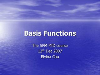
Basis Functions The SPM MfD course 12th Dec 2007 Elvina Chu
Introduction • What is a basis function • What do they do in MRI • How are they useful in SPM
v = 4 i + 2 j j i Basis • Mathematical term to describe any point in space • Euclidian i.e. the x y z co-ordinates y 2 i 4 x
Function • Vectors are produced as each function in the function space can be represented as a linear combination of basis functions. • Linear algebra: Orthonormal i.e. same unit length with perpendicular elements
Uses in SPM • Spatial normalisation to register different subjects to the same co-ordinate system • Ease of reporting in standard space • Useful for reporting what happens generically to individuals in functional imaging
Uses in SPM • Basis functions are used to model the haemodynamic response Finite impulse response Fourier
Fourier Basis • % signal change with time Fourier analysis: the complex wave at the top can be decomposed into the sum of the three simpler waves shown below. f(t)=h1(t)+h2(t)+h3(t) f(t) h1(t) h2(t) h3(t)
Gamma Function Provides a reasonably good fit to the impulse response, although it lacks an undershoot. Fewer functions required to capture the typical range of impulse responses than other sets, thus reducing the degrees of freedom in design matrix
Canonical haemodynamic response function (HRF) Typical BOLD response to an impulse stimulation The response peaks approximately 5 sec after stimulation, and is followed by an undershoot.
Canonical HRF Temporal derivative Dispersion derivative The canonical HRF is a “typical” BOLD impulse response characterised by two gamma functions. Temporal derivative can capture differences in latency of peak response Dispersion derivative can capture differences in duration of peak response
Left Right Mean Design matrix 3 regressors used to model each condition The three basis functions are: 1. Canonical HRF 2. Derivatives with respect to time 3. Derivatives with respect to dispersion
Comparison of the fitted response These plots show the haemodynamic response at a single voxel. The left plot shows the HRF as estimated using the simple model. Lack of fit is corrected, on the right using a more flexible model with basis functions.
Summary • Basis functions identify position in space • Used to model the HRF of BOLD response to an impulse stimulation in fMRI • SPM allows you to choose from 4 different basis functions
Multiple Regression Analysis & Correlated Regressors Hanneke den Ouden Methods for Dummies 2007 12/12/2007
Overview • General • Regression analysis • Multiple regressions • Collinearity / correlated regressors • Orthogonalisation of regressors in SPM
Regression analysis regression analysis examines the relation of a dependent variable Y to specified independent variables X: Y = aX + b • if the model fits the data well: • R2 is high (reflects the proportion of variance in Y explained by the regressor X) • the corresponding p value will be low
Multiple regression analysis • Multiple regression characterises the relationship between several independent variables (or regressors), X1, X2, X3 etc, and a single dependent variable, Y: Y = β1X1 + β2X2 +…..+ βLXL + ε • The X variables are combined linearly and each has its own regression coefficient β (weight) • βs reflect the independent contribution of each regressor, X, to the value of the dependent variable, Y • i.e. the proportion of the variance in Y accounted for by each regressor after all other regressors are accounted for
Multicollinearity • Multiple regression results are sometimes difficult to interpret: • the overall p value of a fitted model is very low • i.e. the model fits the data well • but individual p values for the regressors are high • i.e. none of the X variables has a significant impact on predicting Y. • How is this possible? • Caused when two (or more) regressors are highly correlated: problem known as multicollinearity
Multicollinearity • Are correlated regressors a problem? • No • when you want to predict Y from X1 and X2 • Because R2 and p will be correct • Yes • when you want assess impact of individual regressors • Because individual p values can be misleading: a p value can be high, even though the variable is important • In practice this will nearly always be the case
General Linear Model & Correlated Regressors
General Linear Model and fMRI Y= X. β+ ε Observed data Y is the BOLD signal at various time points at a single voxel • Design matrix • Several components which explain the observed data Y: • Different stimuli • Movement regressors Parameters (or betas) Define the contribution of each component of the design matrix to the value of Y Error (or residuals) Any variance in Y that cannot be explained by the model X.β
Collinearity example • Experiment: • Which areas of the brain are active in reward processing? • Subjects press a button to get a reward when they spot a red dot amongst green dots • model to be fit: Y = β1X1 + β2X2 + ε Y = BOLD response X1 = button press (movement) X2 = response to reward
Collinearity example Which areas of the brain are active in reward processing? • The regressors are linearly dependent (correlated), so • variance attributable to an individual regressor may be confounded with other regressor(s) • As a result we don’t know which part of the BOLD response is explained by movement and which by response to getting a reward • this may lead to misinterpretations of activations in certain brain areas • Primary motor cortex involved in reward processing?? We can’t answer the question
How to deal with collinearity Avoid it: Design the experiment so that the independent variables are uncorrelated • Use common sense • Use toolbox “Design Magic” - Multicollinearity assessment for fMRI for SPM • URL: http://www.matthijs-vink.com/tools.html • Allows you to assess the multicollinearity in your fMRI-design by calculating the amount of factor variance that is also accounted for by the other factors in the design (expressed in R2). • also allows you to reduce correlations between regressors through use of high-pass filters
How to deal with collinearity II • Orthogonalise the correlated regressor variables • using factor analysis (like PCA) • this will produce linearly independent regressors and corresponding factor scores. • these factor scores can subsequently be used instead of the original correlated regressor values • However, the meaning of these factors is rather unclear… so SPM does not do this • Instead SPM does something called serial orthogonalisation • (note that this is only within each condition, so for each condition and its associated parametric modulators, if there are any)
When we have only one regressor, things are simple… Serial Orthogonalisation Y= 1X1 1 = 1.5
When we two correlated regressors, things become difficult… The value of 1 is now smaller, so X1 now explains less of the variance, as X2 explains some of the variance X1 used to explain Serial Orthogonalisation Y= 1X1+2X2 1 = 1 2 = 1
We now orthogonalise X2 with respect to X1, and call this X2* - 1 now again has the original value it had when X2 was not included - 2* is the same value as 2 - X2* is a different regressor from X2!!! Serial Orthogonalisation Y= 1X1+2*X2* 1 = 1.5 2* = 1
Serial Orthogonalisation in SPM • Regressors are orthogonalised from left to right in the design matrix • Order in which you put parametric modulators is important!!! • Put the ‘most important’ modulators first (i.e the ones whose meaning you don’t want to change) • If you add an orthogonalised regressor, the values of the preceding regressors do not change • The regressor you orthogonalise to (X1) does not change • The regressor you are orthogonalising (X2) does change • Plot the orthogonalised regressors to see what it is you are actually estimating
Conclusions • Correlated regressors can be a big problem when analysing / interpreting your data • Try to design your experiment such that you avoid correlated regressors • Estimate how much your regressors are correlated so you know what you’re getting yourself into • If you cannot avoid them • Think about the order of the regressors in your design matrix • Look at what the regressors look like after orthogonalisation
Sources • Will Penny & Klaas Stephan • Rik Henson’s slides: www.mrc-cbu.cam.ac.uk/Imaging/Common/rikSPM-GLM.ppt • Previous years’ presenters’ slides