Radial Basis Functions

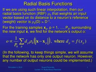
1. Radial Basis Functions If we are using such linear interpolation, then our radial basis function (RBF) 0that weights an input vector based on its distance to a neuron’s reference (weight) vector is 0(D) = D-1. For the training samples xp, p = 1, …, P0, surrounding the new input x, we find for the network’s output o: (In the following, to keep things simple, we will assume that the network has only one output neuron. However, any number of output neurons could be implemented.) Neural Networks Lecture 15: Radial Basis Functions

2. Radial Basis Functions Since it is difficult to define what “surrounding” should mean, it is common to consider all P training samples and use any monotonically decreasing RBF : This, however, implies a network that has as many hidden nodes as there are training samples. This in unacceptable because of its computational complexity and likely poor generalization ability – the network resembles a look-up table. Neural Networks Lecture 15: Radial Basis Functions

3. Radial Basis Functions It is more useful to have fewer neurons and accept that the training set cannot be learned 100% accurately: Here, ideally, each reference vector i of these N neurons should be placed in the center of an input-space cluster of training samples with identical (or at least similar) desired output i. To learn near-optimal values for the reference vectors and the output weights, we can – as usual – employ gradient descent. Neural Networks Lecture 15: Radial Basis Functions

4. The RBF Network output vector o1 • Example: Network function f: R3  R output layer w0 w1 w2 w3 w4 1,1 2,2 3,3 4,4 RBF layer 1 input layer x0=1 x2 x3 input vector Neural Networks Lecture 15: Radial Basis Functions

5. Radial Basis Functions • For a fixed number of neurons N, we could learn the following output weights and reference vectors: • To do this, we first have to define an error function E: • Taken together, we get: Neural Networks Lecture 15: Radial Basis Functions

6. Learning in RBF Networks • Then the error gradient with regard to w1, …, wN is: • For i,j, the j-th vector component of i, we get: Neural Networks Lecture 15: Radial Basis Functions

7. Learning in RBF Networks • The vector length (||…||) expression is inconvenient, because it is the square root of the given vector multiplied by itself. • To eliminate this difficulty, we introduce a function R with R(D2) = (D) and substitute . • This leads to a simplified differentiation: Neural Networks Lecture 15: Radial Basis Functions

8. Learning in RBF Networks Together with the following derivative… … we finally get the result for our error gradient: Neural Networks Lecture 15: Radial Basis Functions

9. Learning in RBF Networks This gives us the following updating rules: where the (positive) learning rates i and i,j could be chosen individually for each parameter wi and i,j. As usual, we can start with random parameters and then iterate these rules for learning until a given error threshold is reached. Neural Networks Lecture 15: Radial Basis Functions

10. Learning in RBF Networks If the node function is given by a Gaussian, then: As a result: Neural Networks Lecture 15: Radial Basis Functions

11. Learning in RBF Networks The specific update rules are now: and Neural Networks Lecture 15: Radial Basis Functions

12. Learning in RBF Networks It turns out that, particularly for Gaussian RBFs, it is more efficient and typically leads to better results to use partially offline training: First, we use any clustering procedure (e.g., k-means) to estimate cluster centers, which are then used to set the values of the reference vectors i and their spreads (standard deviations) i. Then we use the gradient descent method described above to determine the weights wi. Neural Networks Lecture 15: Radial Basis Functions