Radial Basis Function
Radial Basis Function. G.Anuradha. Introduction. RBFN are artificial neural networks for application to problems of supervised learning: Regression Classification Time series prediction. Supervised Learning. A problem that appears in many disciplines

Radial Basis Function
E N D
Presentation Transcript
Radial Basis Function G.Anuradha
Introduction • RBFN are artificial neural networks for application to problems of supervised learning: • Regression • Classification • Time series prediction.
Supervised Learning • A problem that appears in many disciplines • Estimate a function from some example input-output pairs with little (or no) knowledge of the form of the function. • The function is learned from the examples a teacher supplies. The training set:
Parametric Regression • Parametric regression-the form of the function is known but not the parameters values. • Typically, the parameters (both the dependent and independent) have physical meaning. • E.g. fitting a straight line to a bunch of points-
Non Parametric Regression • No priori knowledge of the true form of the function. • Using many free parameters which have no physical meaning. • The model should be able to represent a very broad class of functions.
Classification • Purpose: assign previously unseen patterns to their respective classes. • Training: previous examples of each class. • Output: a class out of a discrete set of classes. • Classification problems can be made to look like nonparametric regression.
Time Series Prediction • Estimate the next value and future values of a sequence, such as: • The problem is that usually it is not an explicit function of time. Normally time series are modeled as autoregressive in nature, i.e. the outputs, suitably delayed, are also the inputs: • To create the training set from the available historical sequence first requires the choice of how many and which delayed outputs affect the next output.
Supervised Learning in RBFN • Neural networks, including radial basis function networks, are nonparametric models and their weights (and other parameters) have no particular meaning in relation to the problems to which they are applied. • Estimating values for the weights of a neural network (or the parameters of any nonparametric model) is never the primary goal in supervised learning. • The primary goal is to estimate the underlying function (or at least to estimate its output at certain desired values of the input).
Basic architecture Hidden layer performs a non-linear mapping from input space into higher dimensional space Gaussian function Weights from the hidden layer are cluster centers
Covers Theorem “A complex pattern-classification problem cast in high-dimensional space nonlinearly is more likely to be linearly separable than in a low dimensional space” (Cover, 1965).
Introduction to Cover’s Theorem • Let X denote a set of N patterns (points) x1,x2,x3,…,xN • Each point is assigned to one of two classes: X+ and X- • This dichotomy is separableif there exist a surface that separates these two classes of points.
Introduction to Cover’s Theorem – Cont’d • For each pattern define the next vector: T • The vector maps points in a p-dimensional input space into corresponding points in a new space of dimension m. • Each is a hidden function, i.e., a hidden unit
Introduction to Cover’s Theorem – Cont’d • A dichotomy {X+,X-} is said to be φ-separableif there exist a m-dimensional vector w such that we may write (Cover, 1965): • wT φ(x) 0, x X+ • wT φ(x) < 0, x X- • The hyperplane defined by wT φ(x) = 0, is the separating surface between the two classes.
RBF Networks for classification • MLP • RBF
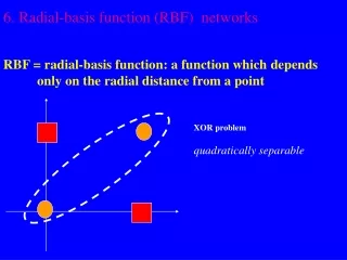
RBF Networks for classification Contd… • An MLP naturally separates the classes with hyperplanes in the Input space • RBF would be to separate class distributions by localizing radial basis functions • Types of separating surfaces are • Hyperplane-linearly separable • Spherically separable-Hypersphere • Quadratically separable-Quadrics
Hyperplane-linearly separable Hypersphere-spherically separable X X X X X X X X Quadratically separable- Quadrics X
What happens in Hidden layer? • The patterns in the input space form clusters • If the centers of these clusters are known then the distance from the cluster center can be measured • The most commonly used radial basis function is a Gaussian function • In a RBF network r is the distance from the cluster centre
center Small Large Gaussian RBF φ φ : is a measure of how spread the curve is:
Distance measure • The distance measured from the cluster centre is usually the Euclidean distance • For each neuron in the hidden layer, the weights represent the co-ordinates from the centre of the cluster • When the neuron receives an input pattern X, the distance is found using the equation
Width of hidden unit 1 2 where Is the width or radius of the bell shape and has to be determined empirically M=no. of basis function Dmax=distance between them =basis function centre 3
Training of the hidden layer • The hidden layer in a RBF network has units which have weights corresponding to the vector representation of the centre of the cluster • These weights are found either by k-means clustering algo or kohonen’s algorithm • Training is unsupervised but the no. of clusters is set in advance. The algorithms finds the best fit to these clusters.
K-means algorithm • Initially ‘k’ points in the pattern space are randomly set • Then for each item of data in the training set, the distances are found from all of the ‘k’ centres • The closest centre is chosen for each item of data. This is the initial classification, so all items of data will be assigned a class from 1 to ‘k’ • Then for all data which has been found to be in class 1, the average or mean values are found for each of the co-ordinates • These become the new values for the centre corresponding to class 1 • This is repeated till class k-which generates k-new centres • This process is repeated until there is no further change
Adaptive k-means algorithm • Similar to kohenen learning. • Input patterns are presented to all of the cluster centers one at a time and the cluster centers adjusted after each one • Cluster center that is nearest to the input data wins, and is shifted slightly towards the new data • Online training can be done using kohenen algo.
Training the output layer • The output layer is trained using the least mean square algorithm, which is a gradient descent technique • Given input signal vector x(n) and desired response d(n) • Set initial weights w(x)=0 • For n=1,2,……….. Compute e(n)=error=d – wtx w(n+1)=w(n)+c.x(n).e(n)
Similarities between RBF and MLP • Both are feedforward • Both are universal approximators • Both are used in similar application areas
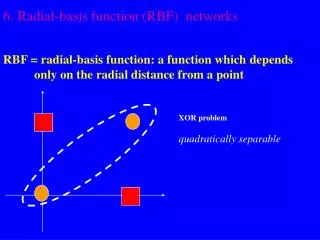
x2 (0,1) (1,1) 0 1 y x1 (0,0) (1,0) Example: the XOR problem • Input space: • Output space: • Construct an RBF pattern classifier such that: (0,0) and (1,1) are mapped to 0, class C1 (1,0) and (0,1) are mapped to 1, class C2
φ2 (0,0) Decision boundary 1.0 0.5 (1,1) 1.0 φ1 0.5 (0,1) and (1,0) Example: the XOR problem • In the feature (hidden layer) space: • When mapped into the feature space < 1 , 2 > (hidden layer), C1 and C2become linearly separable. Soa linear classifier with 1(x) and 2(x) as inputs can be used to solve the XOR problem.
x1 t1 -1 y x2 t2 -1 +1 RBF NN for the XOR problem
RBF network parameters • What do we have to learn for a RBF NN with a given architecture? • The centersof theRBF activation functions • the spreads of the Gaussian RBF activation functions • the weights from the hidden to the output layer • Different learning algorithms may be used for learning the RBF network parameters. We describe three possible methods for learning centers, spreads and weights.
Learning Algorithm 1 • Centers: are selected at random • centers are chosen randomly from the training set • Spreads: are chosen by normalization: • Then the activation function of hidden neuron becomes:
Learning Algorithm 1 • Weights:are computed by means of the pseudo-inverse method. • For an example consider the output of the network • We would like for each example, that is
Learning Algorithm 1 • This can be re-written in matrix form for one example and for all the examples at the same time
Learning Algorithm 1 let then we can write If is the pseudo-inverse of the matrix we obtain the weights using the following formula
Exercise • Check what happens if you choose two different basis function centres
Application: FACE RECOGNITION • The problem: • Face recognition of persons of a known group in an indoor environment. • The approach: • Learn face classes over a wide range of poses using an RBF network.
Dataset • database • 100 images of 10 people (8-bit grayscale, resolution 384 x 287) • for each individual, 10 images of head in different pose from face-on to profile • Designed to asses performance of face recognition techniques when pose variations occur
Datasets All ten images for classes 0-3 from the Sussex database, nose-centred and subsampled to 25x25 before preprocessing
Approach: Face unit RBF • A face recognition unit RBF neural networks is trained to recognize a single person. • Training uses examples of images of the person to be recognized as positive evidence, together with selected confusable images of other people as negative evidence.
Network Architecture • Input layer contains 25*25 inputs which represent the pixel intensities (normalized) of an image. • Hidden layer contains p+a neurons: • p hidden pro neurons (receptors for positive evidence) • ahidden anti neurons (receptors for negative evidence) • Output layer contains two neurons: • One for the particular person. • One for all the others. The output is discarded if the absolute difference of the two output neurons is smaller than a parameter R.
RBF Architecture for one face recognition Output units Linear Supervised RBF units Non-linear Unsupervised Input units
Hidden Layer • Hidden nodes can be: • Pro neurons: Evidence for that person. • Anti neurons: Negative evidence. • The number of pro neurons is equal to the positive examples of the training set. For each pro neuron there is either one or two anti neurons. • Hidden neuron model: Gaussian RBF function.
Training and Testing • Centers: • of a pro neuron: the corresponding positive example • of an anti neuron: the negative example which is most similar to the corresponding pro neuron, with respect to the Euclidean distance. • Spread: average distance of the center from all other centers. So the spread of a hidden neuron n is where H is the number of hidden neurons and is the center of neuron . • Weights: determined using the pseudo-inverse method. • A RBF network with 6 pro neurons, 12 anti neurons, and R equal to 0.3, discarded 23 pro cent of the images of the test set and classified correctly 96 pro cent of the non discarded images.
