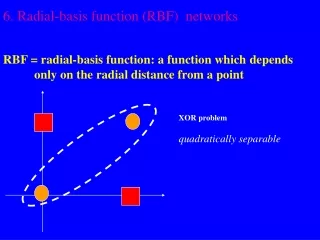
Introduction to Radial Basis Function Networks

1. Introduction to Radial Basis Function Networks

2. Contents • Overview • The Models of Function Approximator • The Radial Basis Function Networks • RBFN’s for Function Approximation • The Projection Matrix • Learning the Kernels • Bias-Variance Dilemma • The Effective Number of Parameters • Model Selection

3. RBF • Linear models have been studied in statistics for about 200 years and the theory is applicable to RBF networks which are just one particular type of linear model. • However, the fashion for neural networks which started in the mid-80 has given rise to new names for concepts already familiar to statisticians

4. Typical Applications of NN • Pattern Classification • Function Approximation • Time-Series Forecasting

5. f ˆ f Function Approximation Unknown Approximator

6. Introduction to Radial Basis Function Networks The Model of Function Approximator

7. Linear Models Weights Fixed Basis Functions

8. y w2 w1 wm 1 2 m x1 x2 xn x = Linear Models Linearly weighted output Output Units • Decomposition • Feature Extraction • Transformation Hidden Units Inputs Feature Vectors

9. Linear Models Can you say some bases? y Linearly weighted output Output Units w2 w1 wm • Decomposition • Feature Extraction • Transformation Hidden Units 1 2 m Inputs Feature Vectors x1 x2 xn x =

10. Example Linear Models Are they orthogonal bases? • Polynomial • Fourier Series

11. y w2 w1 wm 1 2 m x1 x2 xn x = Single-Layer Perceptrons as Universal Aproximators With sufficient number of sigmoidal units, it can be a universal approximator. Hidden Units

12. y w2 w1 wm 1 2 m x1 x2 xn x = Radial Basis Function Networks as Universal Aproximators With sufficient number of radial-basis-function units, it can also be a universal approximator. Hidden Units

13. Non-Linear Models Weights Adjusted by the Learning process

14. Introduction to Radial Basis Function Networks The Radial Basis Function Networks

15. Radial Basis Functions • Center • Distance Measure • Shape Three parameters for a radial function: i(x)= (||x  xi||) xi r = ||x  xi|| 

16. Typical Radial Functions • Gaussian • Hardy-Multiquadratic (1971) • Inverse Multiquadratic

17. Gaussian Basis Function (=0.5,1.0,1.5)

18. Inverse Multiquadratic c=5 c=4 c=3 c=2 c=1

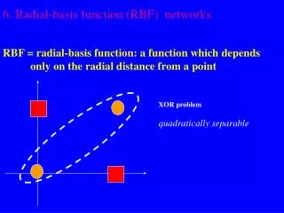
19. + + + Basis {i: i =1,2,…} is `near’ orthogonal. Most General RBF

20. Properties of RBF’s • On-Center, Off Surround • Analogies with localized receptive fields found in several biological structures, e.g., • visual cortex; • ganglion cells

21. y1 ym x1 x2 xn As a function approximator The Topology of RBF Output Units Interpolation Hidden Units Projection Inputs Feature Vectors

22. y1 ym x1 x2 xn As a pattern classifier. The Topology of RBF Output Units Classes Hidden Units Subclasses Inputs Feature Vectors

23. Introduction to Radial Basis Function Networks RBFN’s for Function Approximation

24. Radial Basis Function Networks • Radial basis function (RBF) networks are feed-forward networks trained using a supervised training algorithm. • The activation function is selected from a class of functions called basis functions. • They usually train much faster than BP. • They are less susceptible to problems with non-stationary inputs

25. Radial Basis Function Networks • Popularized by Broomhead and Lowe (1988), and Moody and Darken (1989), RBF networks have proven to be a useful neural network architecture. • The major difference between RBF and BP is the behavior of the single hidden layer. • Rather than using the sigmoidal or S-shaped activation function as in BP, the hidden units in RBF networks use a Gaussian or some other basis kernel function.

26. Unknown Function to Approximate Training Data The idea y x

27. Unknown Function to Approximate Training Data Basis Functions (Kernels) The idea y x

28. Function Learned Basis Functions (Kernels) The idea y x

29. Nontraining Sample Function Learned Basis Functions (Kernels) The idea y x

30. Nontraining Sample Function Learned The idea y x

31. w2 w1 wm x1 x2 xn x = Radial Basis Function Networks as Universal Aproximators Training set Goal for all k

32. w2 w1 wm x1 x2 xn x = Learn the Optimal Weight Vector Training set Goal for all k

33. Regularization Training set If regularization is unneeded, set Goal for all k

34. Learn the Optimal Weight Vector Minimize

35. Learn the Optimal Weight Vector Define

36. Learn the Optimal Weight Vector Define

37. Learn the Optimal Weight Vector

38. Learn the Optimal Weight Vector Design Matrix Variance Matrix

39. Introduction to Radial Basis Function Networks The Projection Matrix

40. Unknown Function The Empirical-Error Vector

41. Unknown Function The Empirical-Error Vector Error Vector

42. If =0, the RBFN’s learning algorithm is to minimizeSSE (MSE). Sum-Squared-Error Error Vector

43. The Projection Matrix Error Vector

44. Introduction to Radial Basis Function Networks Learning the Kernels

45. y1 yl wlml wl1 wl2 w1m w11 w12 2 m 1 x1 x2 xn RBFN’s as Universal Approximators Training set Kernels

46. y1 yl wlml wl1 wl2 w1m w11 w12 2 m 1 x1 x2 xn What to Learn? • Weightswij’s • Centers j’s of j’s • Widthsj’s of j’s • Number of j’s  Model Selection

47. One-Stage Learning

48. The simultaneous updates of all three sets of parameters may be suitable for non-stationary environments or on-line setting. One-Stage Learning

49. y1 yl wlml wl1 wl2 w1m w11 w12 2 m 1 x1 x2 xn Two-Stage Training Determines • Centers j’s of j’s. • Widthsj’s of j’s. • Number of j’s. Step 2 Determines wij’s. E.g., using batch-learning. Step 1

50. Train the Kernels