Download
1 / 36
380 likes | 893 Vues
2806 Neural Computation Radial Basis Function Networks Lecture 5. 2005 Ari Visa. Agenda. Some historical notes Radial Basis Function Networks Some theory Regularization Networks Generalized Radial-Basis Function Networks Approximating properties of RBF Networks Learning Strategies

E N D
2806 Neural ComputationRadial Basis Function Networks Lecture 5 2005 Ari Visa
Agenda • Some historical notes • Radial Basis Function Networks • Some theory • Regularization Networks • Generalized Radial-Basis Function Networks • Approximating properties of RBF Networks • Learning Strategies • Comparison of RBF networks and Multilayer Perceptrons • Conclusions
Some Historical Notes Learning is equivalent to finding a surface in a multidimensional space that provides a best fit to the training data. Powell (1985): Radial-basis functions were introduced in the solution of the real multivariate interpolation problem. Broomhead and Lowe (1988) were the first to exploit the use of radial-basis functions in the design of neural networks. Cover (1965): A pattern-classification problem cast in a high-dimensional space is more likely to be linearly separable than in a low-dimensional space.
Some Historical Notes • Mhaskar, Niyogi and Girosi (1996): The dimension of the hidden space is directly related to the capacity of the network to approximate a smooth input-output mapping (the higher the dimension of the hidden space, the more accurate the approximation will be).
Radial-Basis Function Networks In its most basic form Radial-Basis Function network (RBF) involves three layers with entirely different roles. The input layer is made up of source nodes that connect the network to its environment. The second layer, the only hidden layer, applies a nonlinear transformation from the input space to the hidden space. The output layer is linear, supplying the response of the network to the activation pattern applied to the input layer.
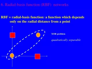
Some Theory • The XOR problem: (x1 OR x2) AND NOT (x1 AND x2)
Some Theory • Cover’s theorem on the separability of patterns (1965): A complex pattern-classification problem cast in a high-dimensional space nonlinearly is more likely to be linearly separable than in a low-dimensional space. Dichotomy = binary partition Let H denote a set of N patterns x1,x2, …,xN. Each of which assigned to one of two classes H1 and H2. (x) = [(x)1. (x)2….(x)m1 ]T A dichotomy {H1 . H2} of H is -separable if there exists am m1-dimensional vector w such that wT(x) > 0, x H1 wT(x) < 0, x H2
Some Theory Separating surfaces: Hyperplanes, quadrices, hypersheres, … P(N,.m1) denote the probability that a particular dictomy picked at random is -separable. Repeated sequence of Bernoulli trials -> E[N] = 2m1 and Median[N]= 2m1 The expected maximum number of randomly assigned patterns that are linearly separable in a space of dimensionality m1 is equal to 2m1.
Some Theory • Interpolation Problem: • Consider a feedforward network with an input layer, a single hidden layer, and an output layer consisting of a single unit. • The network performs a nonlinear mapping from the input space to the hidden layer followed by a linear mapping from the hidden space to the output space • The training phase constitutes the optimization of a fitting procedure for the surface based on known data points presented to the network in the form of input-output examples. • The generalization phase is synonymous with interpolation between the data point, with the interpolation being performed along the constrained surface generated by the fitting procedure as the optimum approximation to the true surface .
Given a set of N different points {xi Rm0 i=1,2,...,N} and a corresponding set of N real numbers {di R1 i=1,2,...,N}, find a function F:RN->R1 that satisfies the interpolation condition F(xi) = di , i=1,2,...,N The radial-basis functions technique consists of choosing a function F F(x) = Ni=1 wi (x-xi ) Some Theory
Some Theory • Micchelli’s Theorem • Let {xi}Ni=1 be a set of distinct points inRm0 . . Then the N-by-N interpolation matrix , whose ji-th element is ij =(xj-xi ) is nonsingular.
Some Theory • The strict interpolation procedure is not a good strategy for the training of RBF networks because of poor generalization to new data. • Learning is viewed as a problem of hyperspace recontruction, given a set of data points that may be sparse. • Two related problems are said to be the inverse of each other if the formulation of each of them requires partial or full knowledge of each other.
Assume a domain X and a range Y taken to be metric space, and that is related by a fixed but unknown mapping f. The problem of reconstructing the mapping f is said to be well-posed if three conditions are satisfied: Existence: For every input vector x H, there does exist an output y=f(x), where y H . Uniqueness: For any pair of input vectors x,t H, we have f(x)=f(t) if, and only if x=t. Continuity: (=stability) for any >0 there exists =() such that the condition x(x,t)< implies that y(f(x),f(t))<, where (.,.) is the symbol for distance between the two arguments in their respective spaces. Some Theory
Some Theory • If any of these conditions is not satisfied, the problem is said to be ill-posed. • An ill-posed problem means that the large data sets may contain a surprisingly small amount of information about the desired solution • Regularisation: how to make an ill-posed problem into a well-posed one.
Some Theory • Regularization (Tikhonov 1963): in the context of a hypersurface reconstruction problem, the basic idea is to stabilize the solution by means of some auxiliary nonnegative function that embeds prior information about the solution. • The most common form of prior information involves the assumption that the input-output mapping function is smooth.
Some Theory • Input signal: xi Rm0 i=1,2,...,N. • Desired response: di R1 i=1,2,...,N. • The approximating function is denoted by F(x). • Standard Error term denoted by Es (F). • Regularizing Term denoted by Ec(F) depends on the geometric properties of the approximating function F(x). D is a linear differential operator. Prior information about the form of the solution is embedded in the operator D, which is problem-dependent. • The quantity to be minimized in regularization theory is given below:
Some Theory • Fréchet differential of the Tikhonov Functional • The principle of regularization may be stated as: • Fréchet differential of a function may be interpreted as the best local linear approximation. • Green’s identity
Some Theory Euler-Lagrange equation for the Tikhonov function E(F) defines a necessary condition for the Tikhonov functional to have an extremum at Fλ(x). The equation represents a partial differential equation in the approximating function F. L = D~D. The minimizing solution Fλ(x) to the regularization problem is a linear superposition of N Green’s function. The xi represents the centers of the expansion, and the weights [di-F(xi)]/λ represent the coefficients of the expansion.
Some Theory Green’s Function: Let G(x,) denote a a function in which both vectors x and appear on equal footing but for different purpose: x as a parameter and as an argument. • For a fixed , G(x,) is a function of x and satisfies the prescriped boundary condition. • Except at the point x = . The derivates of G(x,) with respect to x are all continuous; the number of derivates is determined by the order of the operator L. • With G(x,) considered as a function of x , it satisfies the partial differential equation L G(x,) = 0 everywhere except at the point x = , where it has a singularity. That is L G(x,) = (x - ) where (x - ) is the Dirac delta function positioned at the point x = .
Some Theory • Determination of the Expansion Coefficients • (G + λI)w = d • w = (G + λI) -1d • -> Fλ(x) = Ni=1 wiG(x,xi) • The expansion of the solution in terms of a set of Green’s functions. • The number of Green’s function = the number of examples used in the training process.
Some Theory • If the stabilizer D is both translationally and rotationally invariant -> G(x,xi) = G(||x - xi||) -> strict interpolation An example of a Green’s function is the multivariate Gaussian function
Regularization Networks • The regularization network is a universal approximator • The regularization network has the best approximation property • The solution computed by the regularization network is optimal.
Generalized Radial-Basis Function Networks • When N is large, the one-to-one correspondence between the training input data and the Green’s function produces a regularisation network that may be considered expensive. -> • An approximation of the regularized network.
Generalized Radial-Basis Function Networks • The approach taken involves searching for suboptimal solution in a lower-dimensional space that approximates the regularized solution (Galerkin’s method). F*(x) = m1i=1 wi i(x), where {i(x) | i=1,2,...,m1 N} is a new set of linearly independent basis functions and the wi constitute a new set of weights. We set i(x) = G(x-ti ), i=1,2,... m1 where the set of centers {ti | i=1,2,...,m1} is to be determined. Note that this particular choice of basis functions is the only that guarantees that in the case of m1 = N and xi = ti i=1,2,...,N the correct solution is consistently recovered.
Generalized Radial-Basis Function Networks • F*(x) = m1i=1 wi G(x-ti ) • Minimize the new cost functional E(F*) • Note, that the matrix G is now N-by-m1 and therefore no longer symmetric, and the vector w is m1-by-1.-> • w = G+d, λ=0 where G+ is the pseudoinverse of matrix G (G+ = (G+G)-1GT ).
Generalized Radial-Basis Function Networks • The norm in the approximate solution is ordinarily inteded to be a Euclidean norm. When the individual elements of the input vector x belong to different classes, it is more appropriate to consider a general weighted norm. • ||x||2c =(Cx)T(Cx) where C is an m0-by-m0 norm weighting matrix. -> • F*(x) = m1i=1 wi G(x-ti C) • The weighted norm ~ a) an affine transformation to the original input space. b) follows directly from a generalization of m0-dimensional Laplacian in the definition of the pseudo-differential operator D.
Generalized Radial-Basis Function Networks • The covariance matrix determines the receptive field of G(x-ti C). • (x) = G(x-ti C) –a • We may define three different scenarios pertaining to the covariance matrix and its influence on the shape, size, and orientation of the receptive field.
Generalized Radial-Basis Function Networks • The generalized RBF network differs from the regularization RBF: • The number of nodes in the hidden layer: m1 < N (generalized RBF), N (regularization RBF). • The linear weights associated with the output layer, and the positions of the centers of radial-basis functions and the norm weighting matrix associated with the hidden layer have to be learned (generalized RBF). • The linear weights of the output layer have to be learned (regularization RBF).
Learning Strategies • 1) Fixed Centers Selected at Random - an isotropic Gaussian function whose standard deviation is fixed: G(x-ti ²) = exp(-m1/d²max x-ti ²), i =1,2,.. m1 The linear weights in the output layer of the network should be learned. w = G+d - May require a large training set for a satisfactory level of performance.
Learning Strategies • 2) Self-Organized Selection of Centers • a hybrid learning process: • Self-organizing learning stage estimates appropriate locations for the centers of the radial basis functions in the hidden layer. • Supervised learning stage, which completes the design of the network by estimating the linear weights of the output layer.
Learning Strategies • 3) Supervised Selection of Centers • The centers of the radial basis functions and all other free parameters of the network undergo a supervised learning process (= a gradient descent procedure)
Learning Strategies • 4) Strict Interpolation with Regularization
Approximating properties of RBF Networks • Note that the kernel G:Rm0 R is not required to satisfy the property of radial symmetry.
Approximating properties of RBF Networks • The space of approximating functions attainable with multilayer perceptrons and RBF networks becomes increasingly constrained as the input dimensionality m0 is increased. • The generalization error converges to zero only if the number of hidden units m1 increases more slowly than the size N of the training samples. • For a given size N of training sample, the optimum number of hidden units, m1* behaves as m1* N 1/3. • The RBF network exhibits a rate of approximation O(1/ m1) that is similar to that derived by Barron for the case of a multilayer perceptron with sigmoid activation functions.
Comparison of RBF networks and Multilayer Perceptrons • Radial-basis function networks and multilayer perceptrons are both universal approximators. • For the approximation of a nonlinear input-output mapping, the MLP may require smaller number of parameters than the RBF network for the same degree of accuracy. • Some differences:
Summary • The structure of an RBF network is unusual in that the constitution of its hidden units is entirely different from that of its output units. • Tikhonov’s regularization theory provides a sound mathematical basis for the formulation of RBF networks. • The Green’s function G(x,) plays a central role in the theory.