Chapter 12 - Forecasting
Chapter 12 - Forecasting. Patterns of Demand. Quantity. Time. Patterns of Demand. Figure 12.1. Quantity. Time. (a) Horizontal: Data cluster about a horizontal line. Patterns of Demand. Figure 12.1. Quantity. Time. (b) Trend: Data consistently increase or decrease. Patterns of Demand.

Chapter 12 - Forecasting
E N D
Presentation Transcript
Quantity Time Patterns of Demand Figure 12.1
Quantity Time (a) Horizontal: Data cluster about a horizontal line. Patterns of Demand Figure 12.1
Quantity Time (b) Trend: Data consistently increase or decrease. Patterns of Demand Figure 12.1
Year 1 Quantity | | | | | | | | | | | | J F M A M J J A S O N D Months (c) Seasonal: Data consistently show peaks and valleys. Patterns of Demand Figure 12.1
Year 1 Quantity Year 2 | | | | | | | | | | | | J F M A M J J A S O N D Months Patterns of Demand Figure 12.1 (c) Seasonal: Data consistently show peaks and valleys.
Quantity | | | | | | 1 2 3 4 5 6 Years (c) Cyclical: Data reveal gradual increases and decreases over extended periods. Patterns of Demand Figure 12.1
Time Horizon Medium Term Long Term Short Term (3 months– (more than Application (0–3 months) 2 years) 2 years) Forecast quantity Decision area Forecasting technique Demand Forecast Applications Table 12.1
Time Horizon Medium Term Long Term Short Term (3 months– (more than Application (0–3 months) 2 years) 2 years) Forecast quantity Individual products or services Decision area Inventory management Final assembly scheduling Workforce scheduling Master production scheduling Forecasting Time series technique Causal Judgment Demand Forecast Applications Table 12.1
Time Horizon Medium Term Long Term Short Term (3 months– (more than Application (0–3 months) 2 years) 2 years) Forecast quantity Individual Total sales products or Groups or families services of products or services Decision area Inventory Staff planning management Production Final assembly planning scheduling Master production Workforce scheduling scheduling Purchasing Master production Distribution scheduling Forecasting Time series Causal technique Causal Judgment Judgment Demand Forecast Applications Table 12.1
Time Horizon Medium Term Long Term Short Term (3 months– (more than Application (0–3 months) 2 years) 2 years) Forecast quantity Individual Total sales Total sales products or Groups or families services of products or services Decision area Inventory Staff planning Facility location management Production Capacity Final assembly planning planning scheduling Master production Process Workforce scheduling management scheduling Purchasing Master production Distribution scheduling Forecasting Time series Causal Causal technique Causal Judgment Judgment Judgment Demand Forecast Applications Table 12.1
Y Dependent variable X Independent variable Causal MethodsLinear Regression Figure 12.2
Y Dependent variable X Independent variable Causal MethodsLinear Regression Figure 12.2
Regression equation: Y = a + bX Y Dependent variable X Independent variable Causal MethodsLinear Regression Figure 12.2
Regression equation: Y = a + bX Y Actual value of Y Dependent variable Value of X used to estimate Y X Independent variable Causal MethodsLinear Regression Figure 12.2
Regression equation: Y = a + bX Y Estimate of Y from regression equation Actual value of Y Dependent variable Value of X used to estimate Y X Independent variable Causal MethodsLinear Regression Figure 12.2
Deviation, or error Regression equation: Y = a + bX Y Estimate of Y from regression equation { Actual value of Y Dependent variable Value of X used to estimate Y X Independent variable Causal MethodsLinear Regression Figure 12.2
Sales Advertising Month (000 units) (000 $) 1 264 2.5 2 116 1.3 3 165 1.4 4 101 1.0 5 209 2.0 Causal MethodsLinear Regression Example 12.1
Sales Advertising Month (000 units) (000 $) 1 264 2.5 2 116 1.3 3 165 1.4 4 101 1.0 5 209 2.0 Causal MethodsLinear Regression a = – 8.136 b = 109.229X r = 0.98 r2 = 0.96 syx = 15.61 Example 12.1
300 — 250 — 200 — 150 — 100 — 50 Sales Advertising Month (000 units) (000 $) 1 264 2.5 2 116 1.3 3 165 1.4 4 101 1.0 5 209 2.0 a = – 8.136 b = 109.229X r = 0.98 r2 = 0.96 syx = 15.61 Sales (thousands of units) | | | | 1.0 1.5 2.0 2.5 Advertising (thousands of dollars) Causal MethodsLinear Regression Figure 12.3
300 — 250 — 200 — 150 — 100 — 50 Sales Advertising Month (000 units) (000 $) 1 264 2.5 2 116 1.3 3 165 1.4 4 101 1.0 5 209 2.0 a = – 8.136 b = 109.229X r = 0.98 r2 = 0.96 syx = 15.61 Sales (thousands of units) | | | | 1.0 1.5 2.0 2.5 Advertising (thousands of dollars) Causal MethodsLinear Regression Figure 12.3
300 — 250 — 200 — 150 — 100 — 50 Sales Advertising Month (000 units) (000 $) 1 264 2.5 2 116 1.3 3 165 1.4 4 101 1.0 5 209 2.0 a = – 8.136 b = 109.229X r = 0.98 r2 = 0.96 syx = 15.61 Sales (thousands of units) Y = – 8.136 + 109.229X | | | | 1.0 1.5 2.0 2.5 Advertising (thousands of dollars) Causal MethodsLinear Regression Figure 12.3
300 — 250 — 200 — 150 — 100 — 50 Sales Advertising Month (000 units) (000 $) 1 264 2.5 2 116 1.3 3 165 1.4 4 101 1.0 5 209 2.0 a = – 8.136 b = 109.229X r = 0.98 r2 = 0.96 syx = 15.61 Sales (thousands of units) Y = – 8.136 + 109.229X | | | | 1.0 1.5 2.0 2.5 Advertising (thousands of dollars) Causal MethodsLinear Regression Figure 12.3
300 — 250 — 200 — 150 — 100 — 50 Sales Advertising Month (000 units) (000 $) 1 264 2.5 2 116 1.3 3 165 1.4 4 101 1.0 5 209 2.0 a = – 8.136 b = 109.229X r = 0.98 r2 = 0.96 syx = 15.61 Sales (thousands of units) Y = – 8.136 + 109.229X | | | | 1.0 1.5 2.0 2.5 Forecast for Month 6 X = $1750, Y = – 8.136 + 109.229(1.75) Advertising (thousands of dollars) Causal MethodsLinear Regression Figure 12.3
300 — 250 — 200 — 150 — 100 — 50 Sales Advertising Month (000 units) (000 $) 1 264 2.5 2 116 1.3 3 165 1.4 4 101 1.0 5 209 2.0 a = – 8.136 b = 109.229X r = 0.98 r2 = 0.96 syx = 15.61 Sales (thousands of units) Y = – 8.136 + 109.229X | | | | 1.0 1.5 2.0 2.5 Forecast for Month 6 X = $1750, Y = 183.015, or 183,015 units Advertising (thousands of dollars) Causal MethodsLinear Regression Figure 12.3
300 — 250 — 200 — 150 — 100 — 50 Sales Advertising Month (000 units) (000 $) 1 264 2.5 2 116 1.3 3 165 1.4 4 101 1.0 5 209 2.0 a = – 8.136 b = 109.229X r = 0.98 r2 = 0.96 syx = 15.61 Sales (thousands of units) Y = – 8.136 + 109.229X | | | | 1.0 1.5 2.0 2.5 Advertising (thousands of dollars) Causal MethodsLinear Regression Figure 12.3
300 — 250 — 200 — 150 — 100 — 50 Sales Advertising Month (000 units) (000 $) 1 264 2.5 2 116 1.3 3 165 1.4 4 101 1.0 5 209 2.0 a = – 8.136 b = 109.229X r = 0.98 r2 = 0.96 syx = 15.61 Sales (thousands of units) Y = – 8.136 + 109.229X | | | | 1.0 1.5 2.0 2.5 If current stock = 62,500 units, Production = 183,015 – 62,500 = 120,015 units Advertising (thousands of dollars) Causal MethodsLinear Regression Figure 12.3
Causal MethodsLinear Regression Figure 12.4
Causal MethodsLinear Regression Figure 12.4
Sales Advertising Month (000 units) (000 $) 1 264 2.5 2 116 1.3 3 165 1.4 4 101 1.0 5 209 2.0 Causal MethodsLinear Regression Example 12.1
Sales Advertising Month (000 units) (000 $) 1 264 2.5 2 116 1.3 3 165 1.4 4 101 1.0 5 209 2.0 XY – nXY X 2 – nX 2 a = Y – bX b = Causal MethodsLinear Regression Example 12.1
Sales, Y Advertising, X Month (000 units) (000 $) XYX 2Y 2 1 264 2.5 660.0 6.25 69,696 2 116 1.3 150.8 1.69 13,456 3 165 1.4 231.0 1.96 27,225 4 101 1.0 101.0 1.00 10,201 5 209 2.0 418.0 4.00 43,681 XY – nXY X 2 – nX 2 a = Y – bX b = Causal MethodsLinear Regression Example 12.1
Sales, Y Advertising, X Month (000 units) (000 $) XYX 2Y 2 1 264 2.5 660.0 6.25 69,696 2 116 1.3 150.8 1.69 13,456 3 165 1.4 231.0 1.96 27,225 4 101 1.0 101.0 1.00 10,201 5 209 2.0 418.0 4.00 43,681 Total 855 8.2 1560.8 14.90 164,259 Y = 171 X = 1.64 XY – nXY X 2 – nX 2 a = Y – bX b = Causal MethodsLinear Regression Example 12.1
Sales, Y Advertising, X Month (000 units) (000 $) XYX 2Y 2 1 264 2.5 660.0 6.25 69,696 2 116 1.3 150.8 1.69 13,456 3 165 1.4 231.0 1.96 27,225 4 101 1.0 101.0 1.00 10,201 5 209 2.0 418.0 4.00 43,681 Total 855 8.2 1560.8 14.90 164,259 Y = 171 X = 1.64 1560.8 – 5(1.64)(171) 14.90 – 5(1.64)2 a = Y – bX b = Causal MethodsLinear Regression Example 12.1
Sales, Y Advertising, X Month (000 units) (000 $) XYX 2Y 2 1 264 2.5 660.0 6.25 69,696 2 116 1.3 150.8 1.69 13,456 3 165 1.4 231.0 1.96 27,225 4 101 1.0 101.0 1.00 10,201 5 209 2.0 418.0 4.00 43,681 Total 855 8.2 1560.8 14.90 164,259 Y = 171 X = 1.64 a = Y – bX b = 109.229 Causal MethodsLinear Regression Example 12.1
Sales, Y Advertising, X Month (000 units) (000 $) XYX 2Y 2 1 264 2.5 660.0 6.25 69,696 2 116 1.3 150.8 1.69 13,456 3 165 1.4 231.0 1.96 27,225 4 101 1.0 101.0 1.00 10,201 5 209 2.0 418.0 4.00 43,681 Total 855 8.2 1560.8 14.90 164,259 Y = 171 X = 1.64 a = 171 – 109.229(1.64) b = 109.229 Causal MethodsLinear Regression Example 12.1
Sales, Y Advertising, X Month (000 units) (000 $) XYX 2Y 2 1 264 2.5 660.0 6.25 69,696 2 116 1.3 150.8 1.69 13,456 3 165 1.4 231.0 1.96 27,225 4 101 1.0 101.0 1.00 10,201 5 209 2.0 418.0 4.00 43,681 Total 855 8.2 1560.8 14.90 164,259 Y = 171 X = 1.64 a = – 8.136 b = 109.229 Causal MethodsLinear Regression Example 12.1
Sales, Y Advertising, X Month (000 units) (000 $) XYX 2Y 2 1 264 2.5 660.0 6.25 69,696 2 116 1.3 150.8 1.69 13,456 3 165 1.4 231.0 1.96 27,225 4 101 1.0 101.0 1.00 10,201 5 209 2.0 418.0 4.00 43,681 Total 855 8.2 1560.8 14.90 164,259 Y = 171 X = 1.64 a = – 8.136 b = 109.229 Y = – 8.136 + 109.229(X) Causal MethodsLinear Regression Example 12.1
300 — 250 — 200 — 150 — 100 — 50 Sales, Y Advertising, X Month (000 units) (000 $) XYX 2Y 2 1 264 2.5 660.0 6.25 69,696 2 116 1.3 150.8 1.69 13,456 3 165 1.4 231.0 1.96 27,225 4 101 1.0 101.0 1.00 10,201 5 209 2.0 418.0 4.00 43,681 Total 855 8.2 1560.8 14.90 164,259 Y = 171 X = 1.64 Sales (thousands of units) | | | | 1.0 1.5 2.0 2.5 a = - 8.136 b = 109.229 Advertising (thousands of dollars) Y = – 8.136 + 109.229(X) Causal MethodsLinear Regression Figure 12.3
300 — 250 — 200 — 150 — 100 — 50 Sales, Y Advertising, X Month (000 units) (000 $) XYX 2Y 2 1 264 2.5 660.0 6.25 69,696 2 116 1.3 150.8 1.69 13,456 3 165 1.4 231.0 1.96 27,225 4 101 1.0 101.0 1.00 10,201 5 209 2.0 418.0 4.00 43,681 Total 855 8.2 1560.8 14.90 164,259 Y = 171 X = 1.64 Sales (thousands of units) | | | | 1.0 1.5 2.0 2.5 a = - 8.136 b = 109.229 Advertising (thousands of dollars) Y = – 8.136 + 109.229(X) Causal MethodsLinear Regression Figure 12.3
300 — 250 — 200 — 150 — 100 — 50 Sales, Y Advertising, X Month (000 units) (000 $) XYX 2Y 2 1 264 2.5 660.0 6.25 69,696 2 116 1.3 150.8 1.69 13,456 3 165 1.4 231.0 1.96 27,225 4 101 1.0 101.0 1.00 10,201 5 209 2.0 418.0 4.00 43,681 Total 855 8.2 1560.8 14.90 164,259 Y = 171 X = 1.64 Sales (thousands of units) | | | | 1.0 1.5 2.0 2.5 a = - 8.136 b = 109.229 Advertising (thousands of dollars) Y = – 8.136 + 109.229(X) Causal MethodsLinear Regression Figure 12.3
Sales, Y Advertising, X Month (000 units) (000 $) XYX 2Y 2 1 264 2.5 660.0 6.25 69,696 2 116 1.3 150.8 1.69 13,456 3 165 1.4 231.0 1.96 27,225 4 101 1.0 101.0 1.00 10,201 5 209 2.0 418.0 4.00 43,681 Total 855 8.2 1560.8 14.90 164,259 Y = 171 X = 1.64 Causal MethodsLinear Regression Example 12.1
Sales, Y Advertising, X Month (000 units) (000 $) XYX 2Y 2 1 264 2.5 660.0 6.25 69,696 2 116 1.3 150.8 1.69 13,456 3 165 1.4 231.0 1.96 27,225 4 101 1.0 101.0 1.00 10,201 5 209 2.0 418.0 4.00 43,681 Total 855 8.2 1560.8 14.90 164,259 Y = 171 X = 1.64 nXY – X Y [nX 2 – (X) 2][nY 2 – (Y) 2] r = Causal MethodsLinear Regression Example 12.1
Sales, Y Advertising, X Month (000 units) (000 $) XYX 2Y 2 1 264 2.5 660.0 6.25 69,696 2 116 1.3 150.8 1.69 13,456 3 165 1.4 231.0 1.96 27,225 4 101 1.0 101.0 1.00 10,201 5 209 2.0 418.0 4.00 43,681 Total 855 8.2 1560.8 14.90 164,259 Y = 171 X = 1.64 Causal MethodsLinear Regression r = 0.98 Example 12.1
Sales, Y Advertising, X Month (000 units) (000 $) XYX 2Y 2 1 264 2.5 660.0 6.25 69,696 2 116 1.3 150.8 1.69 13,456 3 165 1.4 231.0 1.96 27,225 4 101 1.0 101.0 1.00 10,201 5 209 2.0 418.0 4.00 43,681 Total 855 8.2 1560.8 14.90 164,259 Y = 171 X = 1.64 r = 0.98 r 2 = 0.96 YX = 15.61 Causal MethodsLinear Regression Example 12.1
Sales, Y Advertising, X Month (000 units) (000 $) XYX 2Y 2 1 264 2.5 660.0 6.25 69,696 2 116 1.3 150.8 1.69 13,456 3 165 1.4 231.0 1.96 27,225 4 101 1.0 101.0 1.00 10,201 5 209 2.0 418.0 4.00 43,681 Total 855 8.2 1560.8 14.90 164,259 Y = 171 X = 1.64 Forecast for Month 6: Advertising expenditure = $1750 Y =- 8.136 + 109.229(1.75) r = 0.98 r 2 = 0.96 YX = 15.61 Causal MethodsLinear Regression Example 12.1

