Remote Sensing - I
Remote Sensing - I. - Optical Range - Image Classification. Image Optimization versus Classification. Landsat-TM of Morocco/Anti-Atlas. Classification Product. Enhanced (optimized) Image Data. Object Space. Feature Space. Result Theme Space. Feature- extraction. Classifier.

Remote Sensing - I
E N D
Presentation Transcript
Remote Sensing - I - Optical Range - Image Classification
Image Optimization versus Classification Landsat-TM of Morocco/Anti-Atlas Classification Product Enhanced (optimized) Image Data
Object Space Feature Space Result Theme Space Feature- extraction Classifier Basic Image Classification Methods • Automated mapping by supervised or un-supervised methods based on training sites or determined Euclidean distance • Used mainly for fast evaluations where statistical data of areal distribution of targets is needed (e.g. crops) Scheme of a computer based classification
Supervised – Unsupervised Methods Un-supervised Supervised • Start with knowledge of class types • Classes are chosen at start • Training regions are created for each class • Ground truth used to verify the training regions • No previous knowledge assumed about data • Tries to spectrally separate the pixels • User has controls over: • Number of classes • Number of Iterations • Convergence thresholds
Class Separation Approaches • Class separation based on Quader-Hyperboxes (Parallelepiped) • Class separation based on Spectral Distances (e.g. Minimum Distance; Maximum Likelihood; Spectral Angle Mapper; Spectral Feature Fitting) • Class separation based on Decision Trees • Class separation based on Additional Informatione.g. Shape, Texture, DEM, Thematic Maps(Expert systems; Artificial Neural Networks; Fuzzy Logic; Support Vector Machines)
Object Space, Feature Space and Clusters Object Space band 4 Feature Space C2 C1 Clusters C1 and C2 band 3
Signatures in 2-dimensional Feature Space Different surface signatures (clusters S, V and W) band 4 V S W band 3
DN Band 3 (0,63 - 0,69 µm) Band 4 (0,76 - 0,9 µm) 20 40 100 120 140 80 60 20 40 60 80 100 DN Grassland, vital Waterbodies Uncultivated Land Grassland, less vital Industrial Fallow Area Sealed Surfaces Forest Urban Materials Dense Buildings Scatterplot and Histograms (band 3 versus band 4) Band 4 Band 3
4 V1 S2 V2 2 W S1 3 Signatures in 3-dimensional Feature Space Different surface signatures (clusters S1/2, V1/2 and W)
100 80 60 40 20 100 80 60 40 20 Water Grassland Water Soil Grassland 1 2 3 4 5 7 1 2 3 4 5 7 100 80 60 40 20 Soil RGB-Display of bands 4/3/2 Histograms of trainings sites in band 4 (0,76-0,90 µm) 1 2 3 4 5 7 RGB-display of bands 3/2/1 Supervised classification – Trainings Sites
100 80 60 40 20 100 80 60 40 20 100 80 60 40 20 Water Grassland, vital Forest 1 2 3 4 5 7 1 2 3 4 5 7 1 2 3 4 5 7 100 80 60 40 20 100 80 60 40 20 100 80 60 40 20 Grassland, less vital Uncultivated Land Urban Materials 1 2 3 4 5 7 1 2 3 4 5 7 1 2 3 4 5 7 100 80 60 40 20 100 80 60 40 20 100 80 60 40 20 Sealed Surface Industrial Area Dense Buildings 1 2 3 4 5 7 1 2 3 4 5 7 1 2 3 4 5 7 'Spectra' of a supervised Classification
Y X Cluster Separation Free Clusters
Y X Grassland, vital Waterbodies Uncultivated Land Grassland, less vital Industrial Fallow Area Sealed Surfaces Forest Urban Materials Dense Buildings Cluster Separation by Quader-Hyperboxes Parallelepiped
Y X Grassland, vital Waterbodies Uncultivated Land Grassland, less vital Industrial Fallow Area Sealed Surfaces Forest Urban Materials Dense Buildings Cluster Separation by spectral DistancesMinimum Distance – Distance to Centroid
Y X Grassland, vital Waterbodies Uncultivated Land Grassland, less vital Industrial Fallow Area Sealed Surfaces Forest Urban Materials Dense Buildings Cluster Separation by spectral DistancesMaximum Likelihood
Target Settlement Field Grass Water Forest Uncultiv. Sum of Classifications Settlement 150 21 0 7 17 30 225 Field 0 730 93 14 115 21 973 Grassland 33 121 320 23 54 43 594 Water 3 18 11 83 8 3 126 Forest 29 81 12 4 350 13 483 Uncultivated 39 8 15 3 11 115 191 Sum of Reference 248 979 451 134 555 225 2592 Confusion Matrix Overall Accuracy = Sum of diagonal entries / Total amount of observations = 1738 / 2592 = 67.4 %.
Unsupervised Classification Algorithms • The two most frequently used algorithms are the K-means and the ISODATAclustering algorithm. Both use the minimum distance approach for cluster separation. • Both of these algorithms are iterative procedures. In general, both of them assign first an arbitrary initial cluster vector. The second step classifies each pixel to the closest cluster. In the third step the new cluster mean vectors are calculated based on all the pixels in one cluster. The second and third steps are repeated until the "change" between the iteration is small. The "change" can be defined in several different ways, either by measuring the distances the mean cluster vector have changed from one iteration to another or by the percentage of pixels that have changed between iterations. • The ISODATA algorithm has some further refinements by splitting and merging of clusters. Clusters are merged if either the number of members (pixel) in a cluster is less than a certain threshold or if the centers of two clusters are closer than a certain threshold. • The ISODATA algorithm is similar to the k-means algorithm with the distinct difference that the ISODATA algorithm allows for different number of clusters while the k-means assumes that the number of clusters is known a priori. http://www.yale.edu/ceo/Projects/swap/landcover/Unsupervised_classification.htm
Unsupervised Classification - I K-means Method 2-D Scatter Plot Band 2 Band 1
Unsupervised Classification – II Initial class means – evenly distributed Parameters: (a) number of classes (b) distance threshold Band 2 Band 1
Unsupervised Classification – III Classification by minimum distance Band 2 Band 1
Unsupervised Classification – IV Classification by minimum distance (after first iteration) Band 2 Band 1
Unsupervised Classification – V Recalculation of new class means (centers) Band 2 Band 1
Unsupervised Classification – VI Second iteration Band 2 Band 1
Unsupervised Classification – VII Stop criteria: (a) maximum iteration (b) number of changed pixels Band 2 Band 1
Unsupervised Classification Results based on different numbers of clusters (ISODATA) 4 Cluster 5 Cluster 6 Cluster
Class 1 Class 2 Class 3 Class 4 Class 5 Class 6 Class 7 Class 1 0 Class 2 45 0 Class 3 60 22 0 Class 4 62 20 18 0 Class 5 82 41 27 22 0 Class 6 94 64 43 57 47 0 Class 7 114 74 62 55 35 69 0 Unsupervised Classification 7 Cluster Matrix of euclidian Distances D = Euclidian Distance n = Number of Bands di = Average grey value of class 'd' in band 'I' ei = Average grey value of class 'e' in band 'I'
Feature Space Vegetation Urban Materials Water Trees Grassland Buildings Industrial Areas Case-I Case-II Chlorophyll ≥ 30µg/l Decidious Trees Coniferous Trees Partially Sealed Surfaces Sealed Surfaces Chlorophyll ≤ 30µg/l Classification based on Decision Tree
Gray Value of Pixels Band 1: 62 Band 2: 23 < 26 Band 3: 22 < 23 Band 4: 12 < 15 Band 5: 9 Band 6: 112 Band 7: 6 Spectral requirements of water class fullfilled Use of spectral Information for Class Composition
Classification based on temporal variations of surface characters to improve accuracy of results Settlement Industrial Area Multitemporal Landsat ETM Scenes Forest Water Grassland Multitemporal Approach
Multitemporal Approach – Crop Separation Standard curve of NDVI NDVI 0,900 winter rye 0,800 winter barley winter wheat 0,700 sugar beet silage maize 0,600 potatoes Reflexion 0,500 0,400 0,300 0,200 0,100 0,000 1-Jan 1-Feb 1-Mrz 1-Apr 1-Mai 1-Jun 1-Jul 1-Aug 1-Sep 1-Okt 1-Nov 1-Dez Date
MOMS-02 Data: Tropical Rainforest – Mindanao/Philippines Maximum Likelihood (MLC) MLC involving topol. Data Merge: I = Pan /HS = 4,2,3 RGB EBIS Texture Analysis ISODATA Clustering Classification Results using different Methods
MOMS-02 Data: Tropical Rainforest – Mindanao/Philippines a • ML Classification • a) without DTM • b) incl. a DTM • Note the impact on • topologically sensitive • classes: • 'Feuchtwald' • 'Sekundärwald' b Classification including a Digital Terrain Model (DTM)
Farmland In Zimbabwe (MOMS-02, Pan) Edge combination ( 1.0, 1.5,…4.0) Region growing result (grey value difference: 10, bottleneck size: 15 pixels) Smoothed original (100 iterations) Region merge (minimum area: 1000 pixels) Automatic Detection of Large Objects (Segmentation)
10 40 80 120 200 160 Detected house plots: Township in Zimbabwe (MOMS-02, pan) Sequence of threshold levels > 1 match > 10 matches > 20 matches Automatic Detection of Small Objects (Thresholding)