Download
1 / 14
140 likes | 233 Vues
Explore the objectives and performance of mapping the magnetic field of the ATLAS Solenoid, including a simple field model, a realistic field model, and the precision of the field mapping machine. Discover insights from the study conducted by Paul S. Miyagawa at the University of Manchester.

E N D
Mapping the Magnetic Field of the ATLAS Solenoid • ATLAS experiment + solenoid • Objectives • Field mapping machine • Simple field model • Machine performance • Realistic field model • Conclusions + future plans Paul S Miyagawa University of Manchester
ATLAS Experiment • LHC will produce proton-proton collisions: • cms energy 14 TeV • 25 ns bunch spacing • 1.1×10¹¹ protons/bunch • design luminosity 1034 cm-2s-1 • ATLAS is a general-purpose detector: • diameter 25 m • length 46 m • overall mass 7000 tonnes IoP Particle Physics 2006
ATLAS Solenoid • Solenoid built from 4 coils welded together to give a single coil: • 1159 turns • length 5.3 m • radius 1.25 m. • Operated at 7600 A to produce an axial field of 2 Tesla at centre of solenoid. • Return current cable runs along surface of solenoid containment vessel. • Cables are routed through a magnetically shielded chimney to the power supply. IoP Particle Physics 2006
Objectives • A useful test of the Standard Model would be measurement of W mass with uncertainty of 25 MeV per lepton type per experiment. • W mass derived from the position of the falling edge of the transverse mass distribution. • Momentum scale will be dominant uncertainty in W mass measurement: • Need to keep uncertainty in momentum down to ~15 MeV. • Measure isolated muon tracks with pT ~ 40 GeV over large range of η: • Uncertainty in energy loss negligible. • Concentrate on alignment and B-field. • Momentum accuracy depends on ∫r(rmax - r)Bzdr : • Field at intermediate radii, as measured by the sagitta, is most important. • Typical sagitta will be ~1 mm: • Limit on silicon alignment, even with infinite statistics and ideal algorithms, will be ~1 μm. • Field mapping team targets an accuracy of 0.05% on sagitta to ensure that B-field measurement is not the limiting factor on momentum accuracy. IoP Particle Physics 2006
Field Mapping Machine • Mapping machine designed and built by team at CERN. • Two propeller arms which rotate in . • Carriage slides in z along rails. • 48 Hall probes on both sides of both arms. • Cross-checks between probes on opposite sides of same arm. • Also have cross-checks between arms. • Machine measures field inside solenoid before Inner Detector installed. • Also have 4 NMR probes permanently fixed to solenoid to set overall scale. • An additional NMR probe fixed to machine carriage. IoP Particle Physics 2006
Simple Field Model • Basis of model is field due to a single coil of nominal dimensions: • Modelled as a series of closed circular loops evenly spaced in z. • Each loop approximated as a series of straight-line segments, and Biot-Savart law applied to each segment. • Added in field due to magnetised iron outside the solenoid (4% of total field). • Model is symmetric in and even in z. IoP Particle Physics 2006
Mapping Machine Simulation • Simulated performance of mapping machine during a typical scan: • Included periodic measurements at calibration points near centre and end of solenoid. • Added various errors to simulated data: • Random measurement errors of solenoid current and B-field. • Random walk drifts of solenoid current and Hall probe measurements. • Random calibration scale and alignment errors of Hall probes. • Displacement and rotation of solenoid field relative to mapping machine axis. • Systematic rotation of Hall probes. IoP Particle Physics 2006
Field Fitting • First, correct for drifts in solenoid current and Hall probe measurements. • Calibrated data fitted with two methods: • Geometrical fit • Sum of simple fields known to obey Maxwell’s equations • Long-thin coil (5 mm longer, 5 mm thinner than nominal) • Short-fat coil (5 mm shorter, 5 mm fatter) • Four terms of Fourier-Bessel series (for magnetisation) • Use Minuit for 2 fit to data • Fit gives information about position, shape, etc of coil • Fourier-Bessel fit • General fit able to describe any field obeying Maxwell’s equations • Uses large number of parameters obtained by direct calculation • Calculate Fourier terms from Bzon outer cylinder • Fit hyperbolic terms to ends of cylinder • Fit Br to find z-independent component of field • Poor fit indicates measurement errors rather than incorrect model • Results from fit used to calculate corrections for Hall probe normalisation and alignment. IoP Particle Physics 2006
Fit Quality • Quality of fit measured by comparing track sagitta in field model with track sagitta in fitted field. • Both fits accurate within target level of 5×10⁻⁴. • Probe normalisation and alignment (PNA) correction improves fits. IoP Particle Physics 2006
Realistic Field Model • Developed realistic field model which makes several improvements over the simple field model. • Modelled the actual current path: • four main coil sections, each as a helical coil • welds between main sections • welds at end of solenoid • return current conductor • Modelled real shape of solenoid: • shrinkage due to cool down • bending due to field excitation IoP Particle Physics 2006
Field from Realistic Model • Comparisons with previous model: • Most adjustments to Bz and Br components are O(10 gauss). • Greatest adjustments are at boundaries (coil ends, weld regions). • See effects of different pitches of each coil section. • Return cable has greatest effect on B component. IoP Particle Physics 2006
Conclusions • Solenoid field mapping team will measure the solenoid magnetic field with a target accuracy of 0.05% on the sagitta. • A propeller-type mapping machine has been designed and built, and its performance simulated. • Two fitting methods (geometrical + Fourier-Bessel) have been developed: • Tests with a simple field model show that both fits meet the target accuracy. • These fits can form the basis for more detailed fits suitable for the actual field. • A realistic field model has been developed and makes several improvements over the simple closed-loop model: • Models the actual current path. • Models real shape of solenoid. • Comparisons made with previous model: • Most adjustments are O(10 gauss). • Greatest adjustments are caused by features of realistic model (coil ends, weld regions, different pitches, return cable). IoP Particle Physics 2006
Future Plans • Study performance of field mapping machine and fitting routines using realistic field model. • Field mapping machine commissioned underground during April + May 2006. • Data taking scheduled for June 2006. • Final field map prepared for September 2006. IoP Particle Physics 2006
Acknowledgements • Martin Aleksa (project coordinator) • Marcello Losasso (engineering design) • Felix Bergsma (Hall probes + motors) • Heidi Sandaker (DAQ) • Steve Snow (NMR probes + software) • John Hart + Paul S Miyagawa (software) IoP Particle Physics 2006