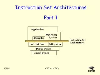
Instruction set architectures
Instruction set architectures. Last time we built a simple, but complete, datapath. The datapath is ultimately controlled by a programmer, so today we’ll look at several aspects of this programming in more detail. How programs are executed on processors

Instruction set architectures
E N D
Presentation Transcript
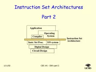
Instruction set architectures • Last time we built a simple, but complete, datapath. • The datapath is ultimately controlled by a programmer, so today we’ll look at several aspects of this programming in more detail. • How programs are executed on processors • An introduction to instruction set architectures • Example instructions and programs • Next, we’ll see how programs are encoded in a processor. Following that, we’ll finish our processor by designing a control unit, which converts our programs into signals for the datapath. ISA
High-level program Compiler Executable file Software Hardware Control Unit Control words Datapath Programming and CPUs • Programs written in a high-level language like C++ must be compiled to produce an executable program. • The result is a CPU-specific machine language program. This can be loaded into memory and executed by the processor. • CS231 focuses on stuff below the dotted blue line, but machine language serves as the interface between hardware and software. ISA
High-level languages • High-level languages provide many useful programming constructs. • For, while, and do loops • If-then-else statements • Functions and procedures for code abstraction • Variables and arrays for storage • Many languages provide safety features as well. • Static and dynamic typechecking • Garbage collection • High-level languages are also relatively portable.Theoretically, you can write one program and compile it on many different processors. • It may be hard to understand what’s so “high-level” here, until you compare these languages with... ISA
Low-level languages • Each CPU has its own low-level instruction set, or machine language, which closely reflects the CPU’s design. • Unfortunately, this means instruction sets are not easy for humans to work with! • Control flow is limited to “jump” and “branch” instructions, which you must use to make your own loops and conditionals. • Support for functions and procedures may be limited. • Memory addresses must be explicitly specified. You can’t just declare new variables and use them! • Very little error checking is provided. • It’s difficult to convert machine language programs to different processors. • Later we’ll look at some rough translations from C to machine language. ISA
Compiling • Processors can’t execute programs written in high-level languages directly, so a special program called a compiler is needed to translate high-level programs into low-level machine code. • In the “good” old days, people often wrote machine language programs by hand to make their programs faster, smaller, or both. • Now, compilers almost always do a better job than people. • Programs are becoming more complex, and it’s hard for humans to write and maintain large, efficient machine language code. • CPUs are becoming more complex. It’s difficult to write code that takes full advantage of a processor’s features. • Some languages, like Perl or Lisp, are usually interpreted instead of compiled. • Programs are translated into an intermediate format. • This is a “middle ground” between efficiency and portability. ISA
Example int main( ){ int a,b,c; scanf ("%d",&a); scanf ("%d",&b); if (a > b) c = a - b; else c = a + b; printf ("c:%d \n", c); } example.c csil:example 4 2 C: 2 gcc -o example example.c gcc -S example.c csil: cat example.s …… ld [%fp+2027], %g4 ld [%fp+2023], %g1 cmp %g4, %g1 ble %icc, .LL2 nop ld [%fp+2027], %g1 ld [%fp+2023], %g4 sub %g1, %g4, %g1 st %g1, [%fp+2019] ba,pt %xcc, .LL3 nop LL2: ld [%fp+2027], %g1 ld [%fp+2023], %g4 add %g1, %g4, %g1 st %g1, [%fp+2019] .LL3: ld [%fp+2019], %g1 ….. ISA
Imagine writing assembly language … Like most of the early hardware and software systems, Fortran waslate in delivery, and didn’t really work when it was delivered. At firstpeople thought it would never be done. Then when it was in fieldtest, with many bugs, and with some of the most important partsunfinished, many thought it would never work. It gradually got to thepoint where a program in Fortran had a reasonable expectancy ofcompiling all the way through and maybe even running. This gradualchange of status from an experiment to a working system was trueof most compilers. It is stressed here in the case of Fortran onlybecause Fortran is now almost taken for granted, as it were built intothe computer hardware. Saul Rosen Programming Languages and Systems McGraw Hill 1967 In late 1953, John W. Backus submitted a proposal to his superiors at IBM to develop a more efficient alternative to assembly language for programming their IBM 704 mainframe computer. … The first manual for FORTRAN appeared in October 1956, with the first FORTRAN compiler delivered in April 1957. From the Wikipedia. ISA
Assembly and machine languages • Machine language instructions are sequences of bits in a specific order. • To make things simpler, people typically use assembly language. • We assign “mnemonic” names to operations and operands. • There is (almost) a one-to-one correspondence between these mnemonics and machine instructions, so it is very easy to convert assembly programs to machine language. • We’ll use assembly code this today to introduce the basic ideas, and switch to machine language next time. ISA
Register transfer instruction: R0 R1 + R2 operation operands ADDR0, R1, R2 destination sources Data manipulation instructions • Data manipulation instructions correspond to ALU operations. • For example, here is a possible addition instruction, and its equivalent using our register transfer notation: • This is similar to a high-level programming statement like R0 = R1 + R2 • Here, all of the operands are registers. ISA
More data manipulation instructions • Here are some other kinds of data manipulation instructions. NOT R0, R1 R0 R1’ ADD R3, R3, #1 R3 R3 + 1 SUB R1, R2, #5 R1 R2 - 5 • Some instructions, like the NOT, have only one operand. • In addition to register operands, constant operands like 1 and 5 are also possible. Constants are denoted with a hash mark in front. ISA
D data WR Write DA D address Register File AA A address B address BA A data B data Constant MB S D1 D0 Q A B FS FS V ALU C N Z F Relation to the datapath • These instructions reflect the design of our datapath from last week. • There are at most two source operands in each instruction, since our ALU has just two inputs. • The two sources can be two registers, or one register and one constant. • More complex operations like R0 R1 + R2 - 3 must be broken down into several lower-level instructions. • Instructions have just one destination operand, which must be a register. ISA
D data WR Write DA D address Register File AA A address B address BA A data B data Constant RAM MB ADRS DATA OUT S D1 D0 Q +5V CS MW WR A B FS FS V ALU C N Z D0 F Q D1 S MD What about RAM? • Recall that our ALU has direct access only to the register file. • RAM contents must be copied to the registers before they can be used as ALU operands. • Similarly, ALU results must go through the registers before they can be stored into memory. • We rely on data movement instructions to transfer data between the RAM and the register file. ISA
A B FS FS V ALU C N Z D0 F Q D1 S Loading a register from RAM • A load instruction copies data from a RAM address to one of the registers. LD R1,(R3) R1 M[R3] • Remember in our datapath, the RAM address must come from one of the registers—in the example above, R3. • The parentheses help show which register operand holds the memory address. D data WR Write DA D address Register File AA A address B address BA A data B data Constant MB S D1 D0 Q RAM ADRS DATA OUT +5V CS MW WR MD ISA
D data WR Write DA D address Register File AA A address B address BA A data B data RAM ADRS DATA OUT +5V CS MW WR A B FS FS V ALU C N Z D0 F Q D1 S Storing a register to RAM • A store instruction copies data from a register to an address in RAM. ST (R3),R1 M[R3] R1 • One register specifies the RAM address to write to—in the example above, R3. • The other operand specifies the actual data to be stored into RAM—R1 above. Constant MB S D1 D0 Q MD ISA
A B FS FS V ALU C N Z D0 F Q D1 S Loading a register with a constant • With our datapath, it’s also possible to load a constant into the register file: LD R1, #0 R1 0 • Our example ALU has a “transfer B” operation (FS=10000) which lets us pass a constant up to the register file. • This gives us an easy way to initialize registers. D data WR Write DA D address Register File AA A address B address BA A data B data Constant MB S D1 D0 Q RAM ADRS DATA OUT +5V CS MW WR MD ISA
D data WR Write DA D address Register File AA A address B address BA A data B data RAM ADRS DATA OUT +5V CS MW WR A B FS FS V ALU C N Z D0 F Q D1 S Storing a constant to RAM • And you can store a constant value directly to RAM too: ST (R3), #0 M[R3] 0 • This provides an easy way to initialize memory contents. Constant MB S D1 D0 Q MD ISA
LD R0, #1000 // R0 1000 LD R0, 1000 // R0 M[1000] LD R3, R0 // R3 R0 LD R3, (R0) // R3 M[R0] The # and ( ) are important! • We’ve seen several statements containing the # or ( ) symbols. These are ways of specifying different addressing modes. • The addressing mode we use determines which data are actually used as operands: • The design of our datapath determines which addressing modes we can use. • The second example above wouldn’t work in our datapath. Why not? • We’ll talk about addressing modes in more detail next week. ISA
LD R0, #1000 // R0 1000 LD R3, (R0) // R3 M[1000] ADD R3, R3, #1 // R3 R3 + 1 ST (R0), R3 // M[1000] R3 A small example • Here’s an example register-transfer operation. M[1000] M[1000] + 1 • This is the assembly-language equivalent: • An awful lot of assembly instructions are needed! • For instance, we have to load the memory address 1000 into a register first, and then use that register to access the RAM. • This is due to our relatively simple datapath design, which only allows register and constant operands to the ALU. • Later on, mostly in CS232, you’ll see why this can be a good thing. ISA
768: LD R0, #1000 // R0 1000 769: LD R3, (R0) // R3 M[1000] 770: ADD R3, R3, #1 // R3 R3 + 1 771: ST (R0), R3 // M[1000] R3 Control flow instructions • Programs consist of a lot of sequential instructions, which are meant to be executed one after another. • Thus, programs are stored in memory so that: • Each program instruction occupies one address. • Instructions are stored one after another. • A program counter (PC) keeps track of the current instruction address. • Ordinarily, the PC just increments after executing each instruction. • But sometimes we need to change this normal sequential behavior, with special control flow instructions. ISA
Jumps • A jump instruction always changes the value of the PC. • The operand specifies exactly how to change the PC. • For simplicity, we often use labels to denote actual addresses. • For example, a program can skip certain instructions. • You can also use jumps to repeat instructions. LD R1, #10 LD R2, #3 JMP L K LD R1, #20 // These two instructions LD R2, #4 // would be skipped L ADD R3, R3, R2 ST (R1), R3 LD R1, #0 F ADD R1, R1, #1 JMP F // An infinite loop! ISA
Branches • A branch instruction may change the PC, depending on whether a given condition is true. LD R1, #10 LD R2, #3 BZ R4, L // Jump to L if R4 == 0 K LD R1, #20 // These instructions may be LD R2, #4 // skipped, depending on R4 L ADD R3, R3, R2 ST (R1), R3 ISA
Types of branches • Branch conditions are often based on the ALU result. • This is what the ALU status bits V, C, N and Z are used for. With them we can implement various branch instructions like the ones below. • Other branch conditions (e.g., branch if greater, equal or less) can be derived from these, along with the right ALU operation. ISA
// Find the absolute value of *X R1 = *X; if (R1 < 0) R1 = -R1; // This might not be executed R3 = R1 + R1; // Sum the integers from 1 to 5 R1 = 0; for (R2 = 1; R2 <= 5; R2++) R1 = R1 + R2; // This is executed five times R3 = R1 + R1; High-level control flow • These jumps and branches are much simpler than the control flow constructs provided by high-level languages. • Conditional statements execute only if some Boolean value is true. • Loops cause some statements to be executed many times ISA
R1 = *X; if (R1 < 0) R1 = -R1; R3 = R1 + R1; LD R1, (X) // R1 = *X BNN R1, L // Skip MUL if R1 is not negative MUL R1, R1, #-1 // R1 = -R1 L ADD R3, R1, R1 // R3 = R1 + R1 Translating the C if-then statement • We can use branch instructions to translate high-level conditional statements into assembly code. • Sometimes it’s easier to invert the original condition. Here, we effectively changed the R1 < 0 test into R1 >= 0. ISA
R1 = 0; for (R2 = 1; R2 <= 5; R2++) R1 = R1 + R2; R3 = R1 + R1; LD R1, #0 // R1 = 0 LD R2, #1 // R2 = 1 FOR BGT R2, #5, L // Stop when R2 > 5 ADD R1, R1, R2 // R1 = R1 + R2 ADD R2, R2, #1 // R2++ JMP FOR // Go back to the loop test L ADD R3, R1, R1 // R3 = R1 + R1 Translating the C for loop • Here is a translation of the for loop, using a hypothetical BGT branch. ISA
Summary • Machine language is the interface between software and processors. • High-level programs must be translated into machine language before they can be run. • There are three main categories of instructions. • Data manipulation operations, such as adding or shifting • Data transfer operations to copy data between registers and RAM • Control flow instructions to change the execution order • Instruction set architectures depend highly on the host CPU’s design. • Today we saw instructions that would be appropriate for our datapath from last week. • Next day we’ll look at some other possibilities. ISA