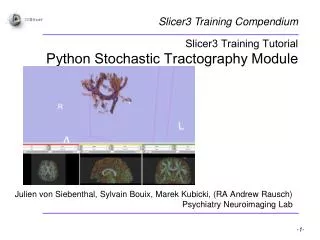
Slicer3 Training Tutorial Python Stochastic Tractography Module
Slicer3 Training Compendium . Slicer3 Training Tutorial Python Stochastic Tractography Module. Julien von Siebenthal, Sylvain Bouix, Marek Kubicki, (RA Andrew Rausch) Psychiatry Neuroimaging Lab. Introduction.

Slicer3 Training Tutorial Python Stochastic Tractography Module
E N D
Presentation Transcript
Slicer3 Training Compendium Slicer3 Training TutorialPython Stochastic Tractography Module Julien von Siebenthal, Sylvain Bouix, Marek Kubicki, (RA Andrew Rausch) Psychiatry Neuroimaging Lab
Introduction • The python stochastic tractography module contains the tools necessary to extract, visualize and quantify white matter connections from DTI images. It seeds nerve fiber bundles from regions of interest (ROIs) based on DWI images. Unlike streamline tractography, stochastic tractography uses a probabilistic framework to perform tractography. • By incorporating uncertainty due to fiber crossings, imaging noise and resolution, stochastic tractography can robustly extract fiber bundles when streamline tractography cannot. • The tracts generated by the stochastic tractography can be used to generate a connectivity probability image, which can be used to study connectivity between different regions of the brain. Rausch, von Siebenthal, Bouix, Kubicki
Materials and Req.’s This course requires the installation of the Slicer3 software and training dataset accessible at the following locations: • Slicer 3 Software (Slicer 3.5 nightly build as of January 3rd, 2010) • http://slicer.org/pages/Special:SlicerDownloads • Training Dataset (packaged and compressed) • http://www.na-mic.org/Wiki/images/0/01/IJdata.tar.gz • Training Wiki • http://www.na-mic.org/Wiki/index.php/Python_Stochastic_Tractography_Tutorial • Prerequisite Skills • Loading images into Slicer 3 Disclaimer It is the responsibility of the user of 3D Slicer to comply with both the terms of the license and with the applicable laws, regulations and rules. Terry, von Siebenthal, Bouix, Kubicki Rausch, von Siebenthal, Bouix, Kubicki
Data This course is built upon three datasets from a single healthy subject brain: DWI (Nrrd) Optional: Whitematter Image (Nrrd) ROI Image(Nrrd) shown overlaid on baseline DWI, tan pixel is seed ROI Terry, von Siebenthal, Bouix, Kubicki Rausch, von Siebenthal, Bouix, Kubicki
ROI Image Regions of Interest (ROI) are denoted by an integer label. An ROI image overlaid on FA image, regions with zero label are transparent. The ROI image is an integer image. Each value defines a unique region. Terry, von Siebenthal, Bouix, Kubicki Rausch, von Siebenthal, Bouix, Kubicki
Learning objective INPUT: DWI, ROI Images Following this tutorial, you’ll be ableto seed nerve fiber bundles and compute a connectivity map using the stochastic tractography module. This map can be used for further analysis. Python Stochastic Tractography Module OUTPUT: Connectivity Map Further Analysis Terry, von Siebenthal, Bouix, Kubicki Rausch, von Siebenthal, Bouix, Kubicki
Enabling Daemons • Also note, if this is your first time using a python module, you must change one slicer setting. • On the top menu, click “View” • Go down to “Application Settings” and select it. • Click the “Slicer Settings” Tab • Click the box to “Slicer Daemon” to enable Slicer Daemons. • You must now close and restart Slicer 3 for these changes to take effect. Terry, von Siebenthal, Bouix, Kubicki Rausch, von Siebenthal, Bouix, Kubicki
Loading Volumes Click the ‘Load Data’ folder button in the upper left part of the program. On the dropdown menu that appears, choose ‘Add data’ Terry, von Siebenthal, Bouix, Kubicki Rausch, von Siebenthal, Bouix, Kubicki
Loading images • In the ‘Add Data’ box that appears, Click Add File(s) • Search file directory for your dwinrrd file. In this tutorial, we will be using namic01-dwi_compressed.nhdr • Click Open • Click Add File(s) again • Search your file directory for ROI file(s). We will use namic01-ROI-corpuscallosum.nhdr • Click Open Terry, von Siebenthal, Bouix, Kubicki Rausch, von Siebenthal, Bouix, Kubicki
Loading ROI • For each image you’re loading, select the ‘Centered’ box • For your ROI, select the ‘LabelMap’ box • If you’re using multiple ROIs, you should load those now the same way, by clicking Add File(s), opening the appropriate nrrd, and checking the Centered and LabelMap options – this is optional, and we won’t do so at this point in the tutorial Terry, von Siebenthal, Bouix, Kubicki Rausch, von Siebenthal, Bouix, Kubicki
Different Data Sets • This module was created on the framework that it could be used by anyone with a diffusion weighted image without external preprocessing steps, therefore making it available to anyone interested in probabilistic tractography. As long as the data can be loaded into Slicer, it can undergo Python Stochastic Tractography. Terry, von Siebenthal, Bouix, Kubicki Rausch, von Siebenthal, Bouix, Kubicki
Verifying the ROI • 1st Click the Rings to link views. • Set B(ackground) as DWI.nhdr image • Set F(oreground) as ROI.nhdr image • Use slider to examine ROI and make sure it is over correct area of DWI. Terry, von Siebenthal, Bouix, Kubicki Rausch, von Siebenthal, Bouix, Kubicki
Verifying the ROI • Slide left and right to examine the position of your ROI in the 3D space of the brain. • In our case, the tan dot is placed centrally in the corpus callosum, just as we expect. Terry, von Siebenthal, Bouix, Kubicki Rausch, von Siebenthal, Bouix, Kubicki
White Matter Mask • A white matter mask is used to include only white matter portions of the brain in tractography to save computation time. • See an example WM Mask by loading namic01-dwi-compressed.nhdr from the tutorial dataset. • If you don’t have a mask for your DWI, the next steps will give us the upper and lower thresholds needed by the Stochastic Tractography module to automatically create one. White matter mask overlaid on DWI baseline image Terry, von Siebenthal, Bouix, Kubicki Rausch, von Siebenthal, Bouix, Kubicki
Extract DWI • Click the Modules drop down tab. • Select Diffusion • Select Diffusion Tensor Estimation Terry, von Siebenthal, Bouix, Kubicki Rausch, von Siebenthal, Bouix, Kubicki
Extract DWI • Click the box next to Input DWI Volume and select namic01-dwi-compressed.nhdr • Click the boxes next to Output DTI Volume, Output Baseline Volume, and Otsu Threshold Mask, and for each option select Create New Volume Terry, von Siebenthal, Bouix, Kubicki Rausch, von Siebenthal, Bouix, Kubicki
Selecting the Baseline • Once this has completed, we will load the baseline for finding our white matter mask thresholds • Set B(ackground) as baseline image, which has lowest number of all the images created. Terry, von Siebenthal, Bouix, Kubicki Rausch, von Siebenthal, Bouix, Kubicki
Thresholding Baseline • Click the Modules drop down tab and select Volumes. • Set the Active Volume to the new Baseline Image. • Adjust the Window/Level values by moving the sliders to make the grey scale image easily viewable Terry, von Siebenthal, Bouix, Kubicki Rausch, von Siebenthal, Bouix, Kubicki
Baseline Intensities • Bright white areas of the ventricles should be excluded • Dark areas outside the brain should also be excluded. • Moving your mouse over the image, find the range of numbers you want to include inside the brain by looking at the ‘Bg’ value shown in the corner of your active axis • Record the upper and lower thresholds for later use. Terry, von Siebenthal, Bouix, Kubicki Rausch, von Siebenthal, Bouix, Kubicki
Launch Stochastic Tractography • Click the Modules drop down tab. • Select Diffusion. • Select Python Stochastic Tractography. Terry, von Siebenthal, Bouix, Kubicki Rausch, von Siebenthal, Bouix, Kubicki
Input/Output Tab • Click Input DWI Volume drop-down menu and select the namic01-dwi-compressed.nhdr • Click Input ROI Volume drop-down menu and select the namic01-ROI-corpuscallosum.nhdr • Optional: • Enter in a second ROI (for filtering) or White Matter Volume Terry, von Siebenthal, Bouix, Kubicki Rausch, von Siebenthal, Bouix, Kubicki
Input/Output Tab • If you would like not only all the tracts coming from one seed ROI, but rather all the tracts coming from one seed ROI that also go though a second ROI, you should select that ROI as your Input ROI Volume (Region B) Terry, von Siebenthal, Bouix, Kubicki Rausch, von Siebenthal, Bouix, Kubicki
Input/Output Tab • If you would prefer to use your own previously generated white matter mask, select Input WM Volume and select your mask. Terry, von Siebenthal, Bouix, Kubicki Rausch, von Siebenthal, Bouix, Kubicki
Smoothing Tab • To enable Gaussian Smoothing, click the box next to Enabled so the check mark is displayed • Enter in FWHM (Full width at half max in millimeters) numbers for each direction. This is the ‘spread’ of the gaussian in the x, y, and z directions. The larger the value the more blurring will occur. Terry, von Siebenthal, Bouix, Kubicki Rausch, von Siebenthal, Bouix, Kubicki
Brain Mask Tab • To enable the mask, click the box next to Enabled so the check mark is displayed • Enter in Lower and Higher brain threshold numbers (based on baseline intensity values). We will use 200-800. • These are the values you determined by looking at the ‘Bg’ values on the extracted baseline. • A wider threshold will include more of the brain, but may take more processing time Terry, von Siebenthal, Bouix, Kubicki Rausch, von Siebenthal, Bouix, Kubicki
IJK/RAS switch • Leave this box checked if your scans are in IJK space. We will check the box for the tutorial. Terry, von Siebenthal, Bouix, Kubicki Rausch, von Siebenthal, Bouix, Kubicki
Diffusion Tensor Tab • Check Enabled as well as FA, TRACE, and/or MODE to output anisotropy index images. Terry, von Siebenthal, Bouix, Kubicki Rausch, von Siebenthal, Bouix, Kubicki
Tractography Tab • Set Total Tracts to the number on tracts you want to be seeded from each ROI voxel. Hundreds are needed to ensure a reliable study. For a quick and dirty tutorial example we’ll use 50. • Set Maximum Tract Length to the length (in mm). For the tutorial, we use 200mm so that no tracts are longer than the length of the brain. • Set Step Size as the distance between each re-estimation of tensors (usually between 0.5 and 1 mm). If this is larger than your voxel size, you can possibly jump over whole slices. In the tutorial, we’ll use 0.8mm. • Check Stopping criteria and enter FA value from 0 to 1 to terminate tracts (e.g. to stop fibers from traveling through the CSF). Normally this is not used in stochastic tractography, and we will not check it in this tutorial. Terry, von Siebenthal, Bouix, Kubicki Rausch, von Siebenthal, Bouix, Kubicki
Connectivity Map Tab • Choose a Computation Mode. • binary (each voxel is counted only once if a fiber passes through it) • cumulative (tracts are summed by voxel independently) We’ll use this setting for the tutorial. • weighted (tracts are summed by voxel depending on their length). • Length Based only shows tracts meeting length criteria. It is not used in this tutorial. • small shows only the shortest 1/3rd of tracts • medium shows only the middle1/3rd • large shows only the longest 1/3rd Terry, von Siebenthal, Bouix, Kubicki Rausch, von Siebenthal, Bouix, Kubicki
Connectivity Map Tab • The remaining options only apply to 2-ROI experiments, and so will not be used in the tutorial. • Threshold between 0 and 1 will cut out tracts that have a lower fraction of tracts on the connectivity map • Tract Offset defines how far back along a tract after its termination the algorithm will search for membership in a second ROI • Use spherical ROI vicinity takes a second ROI and expands it spherically. Useful for very small target ROIs. Vicinity sets the size of the spherical expansion. Terry, von Siebenthal, Bouix, Kubicki Rausch, von Siebenthal, Bouix, Kubicki
Automatic Server Initialisation • In Linux and Mac only, this allows the server running the algorithm to automatically be started Terry, von Siebenthal, Bouix, Kubicki Rausch, von Siebenthal, Bouix, Kubicki
Running Tractography • Now that settings are properly configured, hit Apply to begin tractography. • If a pop-up appears asking to allow external connections from 127.0.0.1, click Yes. Terry, von Siebenthal, Bouix, Kubicki Rausch, von Siebenthal, Bouix, Kubicki
…wait. • Wait until computation is completed. Completed! Rausch, von Siebenthal, Bouix, Kubicki
Module Outputs • Once tractography is complete, it should output 6 new images • brain_### is the mask created by the module • tensor_### is the tensor image • fa_### is an fa map • trace_### is a trace map • mode_### is a mode map • cmFA_### is a normalized connectivity map, where each voxel has a value from 0 to 1 describing the percentage of the total number of tracts that go through this voxel Rausch, von Siebenthal, Bouix, Kubicki
Connectivity Map • The connectivity map is the key output of stochastic tractography, defining a probability of a tract coming from your seed ROI being present at a given point. The image output of stochastic is a grey scale image with values from 0 to 1 describing this probability. Rausch, von Siebenthal, Bouix, Kubicki
Threshold Indication • Scroll over the connectivity map to see its intensity values under “Bg”. You can threshold the connectivity map in the Editor, or examine it in 3D with the Volume Rendering Module. Terry, von Siebenthal, Bouix, Kubicki Rausch, von Siebenthal, Bouix, Kubicki
Saving Outputs • Go to File at the top right corner of the screen and select Save. • Rename the newly created files as you choose and save them in preferred directory. Rausch, von Siebenthal, Bouix, Kubicki
Visualizations • Connectivity files have now been created and can be visualized in 2D or 3D with a couple modules in Slicer. • Editor • VolumeRendering Rausch, von Siebenthal, Bouix, Kubicki
Threshold Label Maps • Go to the Editor from the Modules dropdown menu • Next to Create Label Map From select cmFA_### • Select the Threshold tool • Change the lower bound to 0.1 so that only voxels with a 10% chance of connecting or higher will be included • Press Apply • This label map can be used for label statistics analysis of FA, Mode, etc. Rausch, von Siebenthal, Bouix, Kubicki
Volume Rendering Tab • VolumeRendering will allow you to create a 3D model of your probability cloud. • Drop down the Modules tab and select Volume Rendering. • Under Background Volume, next to Source, select cmFA_###. This will create a probability cloud of the tracts out by stochastic tractography. • If you would like to threshold this cloud to only contain connections with >10% chance of connection, under the Rendering tab, select the Volume Property pane, check the Use Thresholding box to enable, and set the lower value to 0.1. Rausch, von Siebenthal, Bouix, Kubicki
Acknowledgements National Alliance for Medical Image Computing NIH U54EB005149 Morphometry Biomedical Informatics Research Network NIH U24RRO21382 Surgical Planning Laboratory (BWH) Psychiatry Neuroimaging Laboratory Marek Kubicki’s NIH Grant Terry, von Siebenthal, Bouix, Kubicki Rausch, von Siebenthal, Bouix, Kubicki
Appendix • The following images have been generated from either Model Maker or Volume Rendering and modified under Models and Volumes just to show you the many things you can do with your Python Stochastic Tractography Output. • The brain based models are seeded from a corpus callosum ROI from the data of Anna Rotarska-Jagiela at Goethe-Universität. • The helix based models are seeded from an arbitrary ROI from the phantom of Sonia Pujol at BWH. Terry, von Siebenthal, Bouix, Kubicki
Visualize Model Terry, von Siebenthal, Bouix, Kubicki
Glyphs Turned on under Volumes Terry, von Siebenthal, Bouix, Kubicki
Visualize glyphs with models Terry, von Siebenthal, Bouix, Kubicki
Thresholded Terry, von Siebenthal, Bouix, Kubicki
Visualize Tensor (FA) Connectivity Terry, von Siebenthal, Bouix, Kubicki