Tutorial: The Zoltan Toolkit
920 likes | 1.13k Vues
Tutorial: The Zoltan Toolkit. Karen Devine and Cedric Chevalier Sandia National Laboratories, NM Umit Çatalyürek Ohio State University CSCAPES Workshop, June 2008. Outline. High-level view of Zoltan Requirements, data models, and interface Dynamic Load Balancing and Partitioning

Tutorial: The Zoltan Toolkit
E N D
Presentation Transcript
Tutorial: The Zoltan Toolkit Karen Devine and Cedric Chevalier Sandia National Laboratories, NM Umit Çatalyürek Ohio State University CSCAPES Workshop, June 2008
Outline • High-level view of Zoltan • Requirements, data models, and interface • Dynamic Load Balancing and Partitioning • Matrix Ordering • Graph Coloring • Utilities • Alternate Interfaces • Future Directions
Dynamic Load Balancing Graph Coloring G A D H B E C F I 1 0 2 1 2 1 1 0 0 Data Migration Unstructured Communication Distributed Data Directories Matrix Ordering The Zoltan Toolkit • Library of data management services for unstructured, dynamic and/or adaptive computations.
Zoltan System Assumptions • Assume distributed memory model. • Data decomposition + “Owner computes”: • The data is distributed among the processors. • The owner performs all computation on its data. • Data distribution defines work assignment. • Data dependencies among data items owned by different processors incur communication. • Requirements: • MPI • C compiler • GNU Make (gmake)
1 1 1 1 Rg02 Rg2 C02 C2 R 2 R 2 L2 R2 C C 2 2 = 2 1 2 1 1 INDUCTOR R Vs 1 SOURCE_VOLTAGE 1 1 2 Rl Cm012 Cm12 1 A x b R 2 2 C C 2 Rs L1 R1 R Linear solvers & preconditioners 2 2 1 2 1 1 1 INDUCTOR R 1 1 Rg1 Rg01 C01 C1 R R 2 2 C C 2 2 Parallel electronics networks Particle methods Multiphysics simulations Crash simulations Adaptive mesh refinement Zoltan SupportsMany Applications • Different applications, requirements, data structures.
Zoltan Interface Design • Common interface to each class of tools. • Tool/method specified with user parameters. • Data-structure neutral design. • Supports wide range of applications and data structures. • Imposes no restrictions on application’s data structures. • Application does not have to build Zoltan’s data structures.
Zoltan Interface • Simple, easy-to-use interface. • Small number of callable Zoltan functions. • Callable from C, C++, Fortran. • Requirement: Unique global IDs for objects to be partitioned/ordered/colored. For example: • Global element number. • Global matrix row number. • (Processor number, local element number) • (Processor number, local particle number)
Zoltan Application Interface • Application interface: • Zoltan queries the application for needed info. • IDs of objects, coordinates, relationships to other objects. • Application provides simple functions to answer queries. • Small extra costs in memory and function-call overhead. • Query mechanism supports… • Geometric algorithms • Queries for dimensions, coordinates, etc. • Hypergraph- and graph-based algorithms • Queries for edge lists, edge weights, etc. • Tree-based algorithms • Queries for parent/child relationships, etc. • Once query functions are implemented, application can access all Zoltan functionality. • Can switch between algorithms by setting parameters.
APPLICATION ZOLTAN Initialize Zoltan (Zoltan_Initialize, Zoltan_Create) • Zoltan_LB_Partition: • Call query functions. • Build data structures. • Compute new decomposition. • Return import/export lists. COMPUTE Select Method and Parameters (Zoltan_Set_Params) Re-partition (Zoltan_LB_Partition) Register query functions (Zoltan_Set_Fn) Move data (Zoltan_Migrate) • Zoltan_Migrate: • Call packing query functions for exports. • Send exports. • Receive imports. • Call unpacking query functions for imports. Clean up (Zoltan_Destroy) Zoltan Application Interface
Example zoltanSimple.c: ZOLTAN_OBJ_LIST_FN void exGetObjectList(void *userDefinedData, int numGlobalIds, int numLocalIds, ZOLTAN_ID_PTR gids, ZOLTAN_ID_PTR lids, int wgt_dim, float *obj_wgts, int *err) { /* ZOLTAN_OBJ_LIST_FN callback function. ** Returns list of objects owned by this processor. ** lids[i] = local index of object in array. */ int i; for (i=0; i<NumPoints; i++) { gids[i] = GlobalIds[i]; lids[i] = i; } *err = 0; return; }
Example zoltanSimple.c: ZOLTAN_GEOM_MULTI_FN void exGetObjectCoords(void *userDefinedData, int numGlobalIds, int numLocalIds, int numObjs, ZOLTAN_ID_PTR gids, ZOLTAN_ID_PTR lids, int numDim, double *pts, int *err) { /* ZOLTAN_GEOM_MULTI_FN callback. ** Returns coordinates of objects listed in gids and lids. */ int i, id, id3, next = 0; if (numDim != 3) { *err = 1; return; } for (i=0; i<numObjs; i++){ id = lids[i]; if ((id < 0) || (id >= NumPoints)) { *err = 1; return; } id3 = lids[i] * 3; pts[next++] = (double)(Points[id3]); pts[next++] = (double)(Points[id3 + 1]); pts[next++] = (double)(Points[id3 + 2]); } }
More Details on Query Functions • void* data pointer allows user data structures to be used in all query functions. • To use, cast the pointer to the application data type. • Local IDs provided by application are returned by Zoltan to simplify access of application data. • E.g. Indices into local arrays of coordinates. • ZOLTAN_ID_PTRis pointer to array of unsigned integers, allowing IDs to be more than one integer long. • E.g., (processor number, local element number) pair. • numGlobalIds and numLocalIds are lengths of each ID. • All memory for query-function arguments is allocated in Zoltan. void ZOLTAN_GET_GEOM_MULTI_FN(void *userDefinedData, int numGlobalIds, int numLocalIds, int numObjs, ZOLTAN_ID_PTR gids, ZOLTAN_ID_PTR lids, int numDim, double *pts, int *err)
Using Zoltan in Your Application • Decide what your objects are. • Elements? Grid points? Matrix rows? Particles? • Decide which tools (partitioning/ordering/coloring/utilities) and class of method (geometric/graph/hypergraph) to use. • Download Zoltan. • http://www.cs.sandia.gov/Zoltan • Write required query functions for your application. • Required functions are listed with each method in Zoltan User’s Guide. • Call Zoltan from your application. • #include “zoltan.h” in files calling Zoltan. • Edit Zoltan configuration file and build Zoltan. • Compile application; link with libzoltan.a. • mpicc application.c -lzoltan
Partitioning and Load Balancing • Assignment of application data to processors for parallel computation. • Applied to grid points, elements, matrix rows, particles, ….
Partitioning Interface • Zoltan computes the difference (Δ) from current distribution • Choose between: • Import lists (data to import from other procs) • Export lists (data to export to other procs) • Both (the default) • err = Zoltan_LB_Partition(zz, &changes, /* Flag indicating whether partition changed */&numGidEntries, &numLidEntries,&numImport, /* objects to be imported to new part */&importGlobalGids, &importLocalGids, &importProcs, &importToPart, &numExport, /* # objects to be exported from old part */&exportGlobalGids, &exportLocalGids, &exportProcs, &exportToPart);
InitializeApplication PartitionData DistributeData Output& End ComputeSolutions Static Partitioning • Static partitioning in an application: • Data partition is computed. • Data are distributed according to partition map. • Application computes. • Ideal partition: • Processor idle time is minimized. • Inter-processor communication costs are kept low. • Zoltan_Set_Param(zz, “LB_APPROACH”, “PARTITION”);
Dynamic Repartitioning (a.k.a. Dynamic Load Balancing) ComputeSolutions& Adapt • Dynamic repartitioning (load balancing) in an application: • Data partition is computed. • Data are distributed according to partition map. • Application computes and, perhaps, adapts. • Process repeats until the application is done. • Ideal partition: • Processor idle time is minimized. • Inter-processor communication costs are kept low. • Cost to redistribute data is also kept low. • Zoltan_Set_Param(zz, “LB_APPROACH”, “REPARTITION”); InitializeApplication PartitionData RedistributeData Output& End
Zoltan Toolkit:Suite of Partitioners • No single partitioner works best for all applications. • Trade-offs: • Quality vs. speed. • Geometric locality vs. data dependencies. • High-data movement costs vs. tolerance for remapping. • Application developers may not know which partitioner is best for application. • Zoltan contains suite of partitioning methods. • Application changes only one parameter to switch methods. • Zoltan_Set_Param(zz, “LB_METHOD”, “new_method_name”); • Allows experimentation/comparisons to find most effective partitioner for application.
Partitioning Algorithms in the Zoltan Toolkit Geometric (coordinate-based) methods Recursive Coordinate Bisection (Berger, Bokhari) Recursive Inertial Bisection(Taylor, Nour-Omid) Space Filling Curve Partitioning (Warren&Salmon, et al.) Refinement-tree Partitioning (Mitchell) Combinatorial (topology-based) methods Hypergraph Partitioning Hypergraph RepartitioningPaToH (Catalyurek & Aykanat) Zoltan Graph Partitioning ParMETIS (U. Minnesota) Jostle (U. Greenwich)
1st cut 3rd 3rd 2nd 2nd 3rd 3rd Recursive Coordinate Bisection • Zoltan_Set_Param(zz, “LB_METHOD”, “RCB”); • Berger & Bokhari (1987). • Idea: • Divide work into two equal parts using a cutting plane orthogonal to a coordinate axis. • Recursively cut the resulting subdomains.
Geometric Repartitioning • Implicitly achieves low data redistribution costs. • For small changes in data, cuts move only slightly, resulting in little data redistribution.
Adaptive Mesh Refinement Parallel Volume Rendering Crash Simulations and Contact Detection Applications of Geometric Methods Particle Simulations
RCB Advantages and Disadvantages • Advantages: • Conceptually simple; fast and inexpensive. • All processors can inexpensively know entire partition (e.g., for global search in contact detection). • No connectivity info needed (e.g., particle methods). • Good on specialized geometries. • Disadvantages: • No explicit control of communication costs. • Mediocre partition quality. • Can generate disconnected subdomains for complex geometries. • Need coordinate information. SLAC’S 55-cell Linear Accelerator with couplers:One-dimensional RCB partition reduced runtime up to 68% on 512 processor IBM SP3. (Wolf, Ko)
Variations on RCB : Recursive Inertial Bisection • Zoltan_Set_Param(zz, “LB_METHOD”, “RIB”); • Simon, Taylor, et al., 1991 • Cutting planes orthogonal to principle axes of geometry. • Not incremental.
Space-Filling Curve Partitioning (SFC) • Zoltan_Set_Param(zz, “LB_METHOD”, “HSFC”); • Space-Filling Curve (Peano, 1890): • Mapping between R3 to R1 that completely fills a domain. • Applied recursively to obtain desired granularity. • Used for partitioning by … • Warren and Salmon, 1993, gravitational simulations. • Pilkington and Baden, 1994, smoothed particle hydrodynamics. • Patra and Oden, 1995, adaptive mesh refinement.
9 9 6 3 6 3 8 5 2 5 8 4 4 2 7 7 1 1 18 12 10 17 16 13 16 15 14 17 14 12 20 13 15 20 18 10 19 19 11 11 14 12 13 15 9 16 8 11 10 5 6 17 7 4 20 18 1 2 19 3 SFC Algorithm • Run space-filling curve through domain. • Order objects according to position on curve. • Perform 1-D partition of curve.
SFC Advantagesand Disadvantages • Advantages: • Simple, fast, inexpensive. • Maintains geometric locality of objects in processors. • All processors can inexpensively know entire partition (e.g., for global search in contact detection). • Implicitly incremental for repartitioning. • Disadvantages: • No explicit control of communication costs. • Can generate disconnected subdomains. • Often lower quality partitions than RCB. • Geometric coordinates needed.
Applications using SFC • Adaptive hp-refinement finite element methods. • Assigns physically close elements to same processor. • Inexpensive; incremental; fast. • Linear ordering can be used to order elements for efficient memory access. hp-refinement mesh; 8 processors. Patra, et al. (SUNY-Buffalo)
1st cut 1st cut 3rd 3rd 3rd 3rd 2nd 2nd * 2nd 2nd • Determine the part/processor owning region with a given point.Zoltan_LB_Point_PP_Assign • Determine all parts/processors overlapping a given region.Zoltan_LB_Box_PP_Assign 3rd 3rd 3rd 3rd Auxiliary Capabilities for Geometric Methods • Zoltan can store cuts from RCB, RIB, and HSFC inexpensively in each processor. • Zoltan_Set_Param(zz, “KEEP_CUTS”, “1”); • Enables parallel geometric search without communication. • Useful for contact detection, particle methods, rendering.
Graph Partitioning • Zoltan_Set_Param(zz, “LB_METHOD”, “GRAPH”); • Zoltan_Set_Param(zz, “GRAPH_PACKAGE”, “ZOLTAN”); or Zoltan_Set_Param(zz, “GRAPH_PACKAGE”, “PARMETIS”); • Kernighan, Lin, Schweikert, Fiduccia, Mattheyes, Simon, Hendrickson, Leland, Kumar, Karypis, et al. • Represent problem as a weighted graph. • Vertices = objects to be partitioned. • Edges = dependencies between two objects. • Weights = work load or amount of dependency. • Partition graph so that … • Parts have equal vertex weight. • Weight of edges cut by part boundaries is small.
20 20 30 10 10 10 20 10 10 10 30 20 20 Coarsen graph Refine partitionaccounting forcurrent part assignment Partitioncoarse graph Graph Repartitioning • Diffusive strategies (Cybenko, Hu, Blake, Walshaw, Schloegel, et al.) • Shift work from highly loaded processors to less loaded neighbors. • Local communication keeps data redistribution costs low. • Multilevel partitioners that account for data redistribution costs in refining partitions (Schloegel, Karypis) • Parameter weights application communication vs. redistribution communication.
Finite Element Analysis = b A x Linear solvers & preconditioners(square, structurally symmetric systems) Applications using Graph Partitioning Multiphysics andmultiphase simulations
Graph Partitioning:Advantages and Disadvantages • Advantages: • Highly successful model for mesh-based PDE problems. • Explicit control of communication volume gives higher partition quality than geometric methods. • Excellent software available. • Serial: Chaco (SNL) Jostle (U. Greenwich) METIS (U. Minn.) Party (U. Paderborn) Scotch (U. Bordeaux) • Parallel: Zoltan (SNL) ParMETIS (U. Minn.) PJostle (U. Greenwich) • Disadvantages: • More expensive than geometric methods. • Edge-cut model only approximates communication volume.
A A Hypergraph Partitioning Model Graph Partitioning Model Hypergraph Partitioning • Zoltan_Set_Param(zz, “LB_METHOD”, “HYPERGRAPH”); • Zoltan_Set_Param(zz, “HYPERGRAPH_PACKAGE”, “ZOLTAN”); or Zoltan_Set_Param(zz, “HYPERGRAPH_PACKAGE”, “PATOH”); • Alpert, Kahng, Hauck, Borriello, Çatalyürek, Aykanat, Karypis, et al. • Hypergraph model: • Vertices = objects to be partitioned. • Hyperedges = dependencies between two or more objects. • Partitioning goal: Assign equal vertex weight while minimizing hyperedge cut weight.
Hypergraph Repartitioning • Augment hypergraph with data redistribution costs. • Account for data’s current processor assignments. • Weight dependencies by their size and frequency of use. • Partitioning then tries to minimize total communication volume:Data redistribution volume+ Application communication volume Total communication volume • Data redistribution volume: callback returns data sizes. • Zoltan_Set_Fn(zz, ZOLTAN_OBJ_SIZE_MULTI_FN_TYPE, myObjSizeFn, 0); • Application communication volume = Hyperedge cuts * Number of times the communication is done between repartitionings. • Zoltan_Set_Param(zz, “PHG_REPART_MULTIPLIER”, “100”); Best Algorithms Paper Award at IPDPS07 “Hypergraph-based Dynamic Load Balancing for Adaptive Scientific Computations” Çatalyürek, Boman, Devine, Bozdag, Heaphy, & Riesen
1 1 1 1 Rg02 Rg2 C02 C2 2 2 R R 2 L2 R2 C C 2 2 1 2 1 1 INDUCTOR R Vs 1 1 SOURCE_VOLTAGE 1 2 Rl 1 Cm12 Cm012 2 R 2 2 C C Rs L1 R1 R Multiphysics andmultiphase simulations 2 2 1 2 1 1 1 1 1 INDUCTOR R Rg01 Rg1 C01 C1 2 2 R R 2 C C 2 Linear programming for sensor placement Finite Element Analysis = b A x Circuit Simulations Linear solvers & preconditioners(no restrictions on matrix structure) Hypergraph Applications Data Mining
Hypergraph Partitioning:Advantages and Disadvantages • Advantages: • Communication volume reduced 30-38% on average over graph partitioning (Catalyurek & Aykanat). • 5-15% reduction for mesh-based applications. • More accurate communication model than graph partitioning. • Better representation of highly connected and/or non-homogeneous systems. • Greater applicability than graph model. • Can represent rectangular systems and non-symmetric dependencies. • Disadvantages: • Usually more expensive than graph partitioning.
Computation Memory Multi-criteria Load-balancing • Multiple constraints or objectives • Compute a single partition that is good with respect to multiple factors. • Balance both computation and memory. • Balance meshes in loosely coupled physics. • Balance multi-phase simulations. • Extend algorithms to multiple weights • Difficult. No guarantee good solution exists. • Zoltan_Set_Param(zz, “OBJ_WEIGHT_DIM”, “2”); • Available in RCB, RIB and ParMETIS graph partitioning. • In progress in Hypergraphpartitioning.
Entire System ... ... ... Processor Processor Core Core Core Core Heterogeneous Architectures • Clusters may have different types of processors. • Assign “capacity” weights to processors. • E.g., Compute power (speed). • Zoltan_LB_Set_Part_Sizes(…); • Note: Can use this function to specify part sizes for any purpose. • Balance with respect to processor capacity. • Hierarchical partitioning: Allows different partitioners at different architecture levels. • Zoltan_Set_Param(zz, “LB_METHOD”, “HIER”); • Requires three additional callbacks to describe architecture hierarchy. • ZOLTAN_HIER_NUM_LEVELS_FN • ZOLTAN_HIER_PARTITION_FN • ZOLTAN_HIER_METHOD_FN
Sparse Matrix Ordering problem • When solving sparse linear systems with direct methods, non-zero terms are created during the factorization process (A→LLt , A→LDLt or A→LU). • Fill-in depends on the order of the unknowns. • Need to provide fill-reducing orderings.
Fill Reducing ordering • Combinatorial problem, depending on only the structure of the matrix A: • We can work on the graph associated with A. • NP-Complete, thus we deal only with heuristics. • Most popular heuristics: • Minimum Degree algorithms (AMD, MMD, AMF …) • Nested Dissection
A A S B B S Nested dissection (1) • Principle [George 1973] • Find a vertex separator S in graph. • Order vertices of S with highest available indices. • Recursively apply the algorithm to the two separated subgraphs A and B.
Nested dissection (2) • Advantages: • Induces high quality block decompositions. • Suitable for block BLAS 3 computations. • Increases the concurrency of computations. • Compared to minimum degree algorithms. • Very suitable for parallel factorization. • It’s the scope here: parallel ordering is for parallel factorization.
Matrix ordering within Zoltan • Computed by third party libraries: • ParMETIS • Scotch (more specifically PT-Scotch, the parallel part) • Easy to add another one. • The calls to the external ordering library are transparent for the user, and thus Zoltan’s call can be a standard way to compute ordering.