Data Structures – LECTURE Binary search trees
Data Structures – LECTURE Binary search trees. Motivation Operations on binary search trees: Search Minimum, Maximum Predecessor, Successor Insert, Delete Randomly built binary search trees. Motivation: binary search trees.

Data Structures – LECTURE Binary search trees
E N D
Presentation Transcript
Data Structures – LECTURE Binary search trees • Motivation • Operations on binary search trees: • Search • Minimum, Maximum • Predecessor, Successor • Insert, Delete • Randomly built binary search trees
Motivation: binary search trees • A dynamic ADT that efficiently supports the following common operations on S: • Search for an element • Minimum, Maximum • Predecessor, Successor • Insert, Delete • Use a binary tree! All operations take Θ(lg n) • The tree must always be balanced, for otherwise the operations will not take time proportional to the height of the tree!
Binary search tree • A binary search tree has a root, internal nodes with at most two children each, and leaf nodes. • Each node x has the following fields: key(x), left(x), right(x), parent(x) • Binary-search-tree property: Let x be the root of a subtree, and y a node below it. • left subtree: key(y) ≤key(x) • right subtree: key(y) >key(x)
5 2 7 3 5 2 8 5 8 7 Examples of binary trees 3 5 In-order, pre-order, and post-order traversal
Tree-Search routine Tree-Search(x,k)ifx = nullork = key[x]then returnxifk < key[x] then return Tree-Search(left[x],k)elsereturn Tree-Search(right[x],k)Iterative-Tree-Search(x,k)whilex ≠nullandk ≠key[x]do ifk < key[x] then x left[x]elsex right[x]returnx Complexity: O(h) h = tree height
Example: search in a binary tree Search for 13 in the tree
Tree traversal Inorder-Tree-Walk(x)ifx ≠null then Inorder-Tree-Walk(left[x]) print key[x] Inorder-Tree-Walk(right[x]) Recurrence equation: T(0) = Θ(1) T(n) = T(k) + T(n – k –1) + Θ(1) Complexity: Θ(n)
Tree-Minimum(x)whileleft[x] ≠nulldox left[x]returnxTree-Maximum(x)whileright[x] ≠nulldox right[x]returnx Max and Min-Search routines Complexity: O(h)
Tree-Successor routine (1) • The successor of x is the smallest elementy with a key greater than that of x • The successor of x can be found without comparing the keys. It is either: • null if x is the maximum node. • the minimum of the right child of t when t has a right child. • or else, the lowest ancestor of x whose left child is also an ancestor of x.
z x y x Lowest ancestor z of x whose left child y is also an ancestor of x Tree-Successor: cases Minimum of right child of x
Tree-Successor routine (2) Tree-Successor(x)ifright[x] ≠null /* Case 2then return Tree-Minimum(right[x]) y parent[x]while y≠null andx = right[y] /* Case 3 do x y y parent[y] returny
Example: finding a successor Find the successors of 15, 13
Proof (1) • Case 1 is trivial; Case 2 is easy. • Case 3: If x doesn’t have a right child, then its successor is x’s first ancestor such that its left child is also an ancestor of x. (This includes the case that there is no such ancestor, and then x is the maximum and the successor is null.) • Proof: To prove that a node z is the successor of x, we need to show that key[z] > key[x] and that x is the maximum of all elements smaller than z. • Start from x and climb up the tree as long as you move from a right child up. Let the node you stopped at be y, and denote z = parent[y].
Proof (2) • Sub-claim: x is the max of the sub-tree rooted at y. • Proof of sub-claim: x is the node you reach if you go right all the time from y. • Now we claim z = parent(y) is the successor of x. First, key[z] > key[x] because y is the left child of z by the definition of y, so x is in z’s left sub-tree. • Now, x is the maximum of all items that are smaller than z, because by the sub-claim x is the maximum of the sub-tree rooted at y, and all elements smaller than z are in this subtree by the property of binary search trees.
Insert • Insert is very similar to search: find the place in the tree where we want to insert the new node z. • The new node z will always be a leaf. • Initially, assume that left(z) and right(z) are both null.
12 15 18 17 2 19 z 13 Example: insertion 5 9 Insert 13 in the tree
Tree-insert routine Tree-Insert(T,z) y null x root[T] whilex≠null doy x if key[z] < key[x] then x left[x] elsex right[x] parent[z] y y is the parent of x /* When the tree is empty ify = nullthen root[T] z elseifkey[z] < key[y] thenleft[y] z elseright[y] z
Delete Delete is more complicated than insert. There are three cases to delete node z: • z has no children • z has one child • z has two children Case 1: delete z, update the child’s parent child to null. Case 2: delete z and connect its parent to its child. Case 3: more complex. We can’t just take the node out and reconnect its parent with its children, because the tree will no longer be a binary tree!
Delete case 1: no children! delete delete
Delete case 2: one child delete
Delete case 3: two children Replace the node by its successor, and “pull” the successor, which necessarily has at most one child Claim: if a node has two children, its successor has at most one child. Proof: This is because if the node has two children, its successor is the minimum of its right subtree. This minimum cannot have a left child because then the child would be the minimum… Invariant: in all cases the binary search tree property is preserved after the deletion.
Delete z y δ α β w Delete: case 3 proof z δ α β y w
Delete: case 3 delete successor
Tree-Delete routine Tree-Delete(T,z) ifleft[z] = nullorright[z] = null /* Cases 1 or 2 theny z /* find a node y to splice elsey Tree-Successor(z) /* to splice out ifleft[y] ≠null /* set the child x thenx left[y] elsex right[y] ifx ≠null /* splicing operation thenparent[x] parent[y] if parent[y] = null thenroot[T] x elseify = left[parent[y]] then left[parent[y]] x elseright[parent[y]] x /* copy y’s satellite data into z ify ≠z thenkey[z] key[y] returny
Complexity analysis • Delete: The two first cases take O(1) operations: they involve switching the pointers of the parent and the child (if it exists) of the node that is deleted. • The third case requires a call to Tree-Successor, and thus can take O(h) time. • Conclusion: all dynamic operations on a binary search tree take O(h), where h is the tree height. • In the worst case, the height of the tree can be O(n)
Randomly-built Binary Search Trees • Definition: A randomly-built binary search tree over n distinct keys is a binary search tree that results from inserting the n keys in random order (each permutation of the keys is equally likely) into an initially empty tree. • Theorem: The average height of a randomly-built binary search tree of n distinct keys is O(lg n) • Corollary: The dynamic operations Successor, Predecessor, Search, Min, Max, Insert, and Delete all have O(lg n) average complexity on randomly-built binary search trees.