Download
1 / 40
400 likes | 441 Vues
Lecture 6 Smoothing II. CSCE 771 Natural Language Processing. Topics Overview Readings: Chapters. February 4, 2013. Overview. Last Time Tagging Markov Chains Hidden Markov Models NLTK book – chapter 5 tagging Today Viterbi dynamic programming calculation Noam Chomsky on You Tube

E N D
Lecture 6 Smoothing II CSCE 771 Natural Language Processing • Topics • Overview • Readings: Chapters February 4, 2013
Overview • Last Time • Tagging • Markov Chains • Hidden Markov Models • NLTK book – chapter 5 tagging • Today • Viterbi dynamic programming calculation • Noam Chomsky on You Tube • Revisited smoothing • Dealing with zeroes • Laplace • Good-Turing
HMM Review from last time • Tagging • Markov Chains – state known • Hidden Markov Models – states unknown but observations with probabilities state • NLTK book – chapter 5 tagging
Notes on Notation in Virterbi • Viterbi Algorithm • Dynamic programming maximize probability of tag sequence • Argmax • Matrix of probabilities viterbi(state, time) = vs(t) (in 5.18) • Calculate left to right • Bottom to top (states) • Assume vs(t) depend only on • vi(t-1) (previous probabilities) and • aij - the transitional probability state i state j • bj(ot) – observational prob of word ot being in state bj
Figure 5.18 - Viterbi Example Speech and Language Processing - Jurafsky and Martin
Chomsky on You-tube http://www.youtube.com/watch?v=8mA4HYTO790
Smoothing Review • Because our HMM models really needs to count bigrams, trigrams etc. • Zero counts • Laplace = plus 1 • Good-Turing – Ncthe number of words with count c • Simple Good_Turing • Katz-backoff
Speech and Language Processing - Jurafsky and Martin Evaluation of • Standard method • Train parameters of our model on a training set. • Look at the models performance on some new data • This is exactly what happens in the real world; we want to know how our model performs on data we haven’t seen • So use a test set. A dataset which is different than our training set, but is drawn from the same source • Then we need an evaluation metric to tell us how well our model is doing on the test set. • One such metric is perplexity
Unknown Words • But once we start looking at test data, we’ll run into words that we haven’t seen before (pretty much regardless of how much training data you have. • With an Open Vocabulary task • Create an unknown word token <UNK> • Training of <UNK> probabilities • Create a fixed lexicon L, of size V • From a dictionary or • A subset of terms from the training set • At text normalization phase, any training word not in L changed to <UNK> • Now we count that like a normal word • At test time • Use UNK counts for any word not in training Speech and Language Processing - Jurafsky and Martin
Shakespeare as a Corpus • N=884,647 tokens, V=29,066 • Shakespeare produced 300,000 bigram types out of V2= 844 million possible bigrams... • So, 99.96% of the possible bigrams were never seen (have zero entries in the table) • This is the biggest problem in language modeling; we’ll come back to it. • Quadrigrams are worse: What's coming out looks like Shakespeare because it is Shakespeare Speech and Language Processing - Jurafsky and Martin
Zero Counts • Some of those zeros are really zeros... • Things that really can’t or shouldn’t happen. • On the other hand, some of them are just rare events. • If the training corpus had been a little bigger they would have had a count (probably a count of 1!). • Zipf’s Law (long tail phenomenon): • A small number of events occur with high frequency • A large number of events occur with low frequency • You can quickly collect statistics on the high frequency events • You might have to wait an arbitrarily long time to get valid statistics on low frequency events • Result: • Our estimates are sparse! We have no counts at all for the vast bulk of things we want to estimate! • Answer: • Estimate the likelihood of unseen (zero count) N-grams! Speech and Language Processing - Jurafsky and Martin
Laplace Smoothing • Also called add-one smoothing • Just add one to all the counts! • MLE estimate: • Laplace estimate: • Reconstructed counts: Speech and Language Processing - Jurafsky and Martin
Laplace-Smoothed Bigram Probabilities Speech and Language Processing - Jurafsky and Martin
Reconstituted Counts Speech and Language Processing - Jurafsky and Martin
Big Change to the Counts! • C(count to) went from 608 to 238! • P(to|want) from .66 to .26! • Discount d= c*/c • d for “chinese food” =.10!!! A 10x reduction • So in general, Laplace is a blunt instrument • Could use more fine-grained method (add-k) • But Laplace smoothing not used for N-grams, as we have much better methods • Despite its flaws Laplace (add-k) is however still used to smooth other probabilistic models in NLP, especially • For pilot studies • in domains where the number of zeros isn’t so huge. Speech and Language Processing - Jurafsky and Martin
Better Smoothing • Intuition used by many smoothing algorithms • Good-Turing • Kneser-Ney • Witten-Bell • Is to use the count of things we’ve seen once to help estimate the count of things we’ve never seen Speech and Language Processing - Jurafsky and Martin
Good-Turing Josh Goodman Intuition • Imagine you are fishing • There are 8 species: carp, perch, whitefish, trout, salmon, eel, catfish, bass • You have caught • 10 carp, 3 perch, 2 whitefish, 1 trout, 1 salmon, 1 eel = 18 fish • How likely is it that the next fish caught is from a new species (one not seen in our previous catch)? • 3/18 • Assuming so, how likely is it that next species is trout? • Must be less than 1/18 Speech and Language Processing - Jurafsky and Martin
Good-Turing • Notation: Nx is the frequency-of-frequency-x • So N10=1 • Number of fish species seen 10 times is 1 (carp) • N1=3 • Number of fish species seen 1 is 3 (trout, salmon, eel) • To estimate total number of unseen species • Use number of species (words) we’ve seen once • c0* =c1p0 = N1/N • All other estimates are adjusted (down) to give probabilities for unseen Speech and Language Processing - Jurafsky and Martin
Good-Turing Intuition • Notation: Nx is the frequency-of-frequency-x • So N10=1, N1=3, etc • To estimate total number of unseen species • Use number of species (words) we’ve seen once • c0* =c1p0 = N1/N p0=N1/N=3/18 • All other estimates are adjusted (down) to give probabilities for unseen Speech and Language Processing - Jurafsky and Martin
GT Fish Example Speech and Language Processing - Jurafsky and Martin
Bigram Frequencies of Frequencies and GT Re-estimates Speech and Language Processing - Jurafsky and Martin
Complications • In practice, assume large counts (c>k for some k) are reliable: • That complicates c*, making it: • Also: we assume singleton counts c=1 are unreliable, so treat N-grams with count of 1 as if they were count=0 • Also, need the Nk to be non-zero, so we need to smooth (interpolate) the Nk counts before computing c* from them Speech and Language Processing - Jurafsky and Martin
Backoff and Interpolation • Another really useful source of knowledge • If we are estimating: • trigram p(z|x,y) • but count(xyz) is zero • Use info from: • Bigram p(z|y) • Or even: • Unigram p(z) • How to combine this trigram, bigram, unigram info in a valid fashion? Speech and Language Processing - Jurafsky and Martin
Backoff Vs. Interpolation • Backoff: use trigram if you have it, otherwise bigram, otherwise unigram • Interpolation: mix all three Speech and Language Processing - Jurafsky and Martin
Interpolation • Simple interpolation • Lambdas conditional on context:
How to Set the Lambdas? • Use a held-out, or development, corpus • Choose lambdas which maximize the probability of some held-out data • I.e. fix the N-gram probabilities • Then search for lambda values • That when plugged into previous equation • Give largest probability for held-out set • Can use EM to do this search
Why discounts P* and alpha? • MLE probabilities sum to 1 • So if we used MLE probabilities but backed off to lower order model when MLE prob is zero • We would be adding extra probability mass • And total probability would be greater than 1
Intuition of Backoff+Discounting • How much probability to assign to all the zero trigrams? • Use GT or other discounting algorithm to tell us • How to divide that probability mass among different contexts? • Use the N-1 gram estimates to tell us • What do we do for the unigram words not seen in training? • Out Of Vocabulary = OOV words
OOV words: <UNK> word • Out Of Vocabulary = OOV words • We don’t use GT smoothing for these • Because GT assumes we know the number of unseen events • Instead: create an unknown word token <UNK> • Training of <UNK> probabilities • Create a fixed lexicon L of size V • At text normalization phase, any training word not in L changed to <UNK> • Now we train its probabilities like a normal word • At decoding time • If text input: Use UNK probabilities for any word not in training
Practical Issues • We do everything in log space • Avoid underflow • (also adding is faster than multiplying)
Back to Tagging • Brown Tagset - • In 1967, Kucera and Francis published their classic work Computational Analysis of Present-Day American English – • tags added later ~1979 • 500 texts each roughly 2000 words • Zipf’s Law – “the frequency of the n-th most frequent word is roughly proportional to 1/n” • Newer larger corpora ~ 100 million words • Corpus of Contemporary American English, • the British National Corpus or • the International Corpus of English http://en.wikipedia.org/wiki/Brown_Corpus
Figure 5.4 pronoun in Celex Counts from COBUILD 16-million word corpus
Figure 5.18 - Viterbi Example Revisited Speech and Language Processing - Jurafsky and Martin
5.5.4 Extending HMM to Trigrams • Find best tag sequence • Bayes rule • Markov assumption • Extended for Trigrams