From Randomness to Probability
From Randomness to Probability. Chapter 14. A random phenomenon is a situation in which we know what outcomes could happen, but we don’t know which particular outcome did or will happen. In general, each occasion upon which we observe a random phenomenon is called a trial .

From Randomness to Probability
E N D
Presentation Transcript
From Randomness to Probability Chapter 14
A random phenomenon is a situation in which we know what outcomes could happen, but we don’t know which particular outcome did or will happen. In general, each occasion upon which we observe a random phenomenon is called a trial. At each trial, we note the value of the random phenomenon, and call it an outcome. When we combine outcomes, the resulting combination is an event. The collection of all possible outcomes is called the sample space. Dealing with Random Phenomena
Definitions Probability is the mathematics of chance. It tells us the relative frequency with which we can expect an event to occur The greater the probability the more likely the event will occur. It can be written as a fraction, decimal, percent, or ratio.
1 Certain .5 50/50 0 Impossible Definitions Probability is the numerical measure of the likelihood that the event will occur. Value is between 0 and 1. Sum of the probabilities of all events is 1.
Definitions A probability experiment is an action through which specific results (counts, measurements, or responses) are obtained. The result of a single trial in a probability experiment is an outcome. The set of all possible outcomes of a probability experiment is the sample space, denoted as S. e.g. All 6 faces of a die: S = { 1 , 2 , 3 , 4 , 5 , 6 }
Definitions Other Examples of Sample Spaces may include: Lists Lattice Diagrams Venn Diagrams Tree Diagrams May use a combination of these. Where appropriate always display your sample space.
Definitions An event consists of one or more outcomes and is a subset of the sample space. Events are often represented by uppercase letters, such as A, B, or C. Notation: The probability that event E will occur is written P(E) and is read “the probability of event E.”
Number of Event Outcomes P(E) = Total Number of Possible Outcomes in S Definitions • The Probability of an Event, E: • Consider a pair of Dice • Each of the Outcomes in the Sample Space are randomand equally likely to occur. (There are 2 ways to get one 6 and the other 4) e.g. P( ) =
Number of Event Outcomes P(E) = Total Number of Possible Outcomes in S Definitions There are three types of probability 1. Theoretical Probability Theoretical probability is used when each outcome in a sample space is equally likely to occur. The Ultimate probability formula
Theoretical Probability Probabilities determined using mathematical computations based on possible results, or outcomes. This kind of probability is referred to as theoretical probability.
Number of Event Occurrences P(E) = Total Number of Observations Definitions There are three types of probability 2. Experimental Probability (or Empirical Probability) Experimental probability is based upon observations obtained from probability experiments. The experimental probability of an event E is the relative frequency of event E
Experimental Probability Probabilities determined from repeated experimentation and observation, recording results, and then using these results to predict expected probability. This kind of probability is referred to as experimental probability. Also known as Relative Frequency.
Definitions There are three types of probability 3. Personal Probability Personal probability is a probability measure resulting from intuition, educated guesses, and estimates. Therefore, there is no formula to calculate it. Usually found by consulting an expert.
Theoretical vs. Experimental Probability • Related by The Law of Large Numbers. • The Law of Large Numbers: States that the long-run relative frequency (experimental probability) of repeated independent events gets closer and closer to the theoretical probability as the number of trials increases. • Independent - Roughly speaking, this means that the outcome of one trial doesn’t influence or change the outcome of another. • For example, coin flips are independent.
Definitions Law of Large Numbers As an experiment is repeated over and over, the experimental probability of an event approaches the theoretical probability of the event. The greater the number of trials the more likely the experimental probability of an event will equal its theoretical probability.
Example: Theoretical vs. Experimental Probability In the long run, if you flip a coin many times, heads will occur about ½ of the time.
Theoretical vs. Experimental Probability Theoretical Probability – What should occur or happen. Experimental Probability – What actually occurred or happened (relative frequency).
The LLN says nothing about short-run behavior. Relative frequencies even out only in the long run, and this long run is really long (infinitely long, in fact). The so called Law of Averages (that an outcome of a random event that hasn’t occurred in many trials is “due” to occur) doesn’t exist at all. The Nonexistent Law of Averages
We are dealing with probabilities now, not data, but the three rules don’t change. Make a picture. Make a picture. Make a picture. The First Three Rules of Working with Probability
All the pictures we use help us indentify the sample space. Once all possible outcomes have been indentified, calculating the probability of an event is: Pictures: Lists Lattice Diagrams Venn Diagrams Tree Diagrams Number of Event Outcomes P(E) = Total Number of Possible Outcomes in S The First Three Rules of Working with Probability
Two requirements for a probability: A probability is a number between 0 and 1. For any event A, 0 ≤ P(A) ≤ 1. Formal Probability (Laws of Probability)
Probability Assignment Rule: The probability of the set of all possible outcomes of a trial must be 1. P(S) = 1 (S represents the set of all possible outcomes.) Formal Probability
Complement Rule: The set of outcomes that are not in the event A is called the complement of A, denoted AC. The probability of an event occurring is 1 minus the probability that it doesn’t occur: P(A) = 1 – P(AC) Formal Probability
Addition Rule: Events that have no outcomes in common (and, thus, cannot occur together) are called disjoint(or mutually exclusive). Formal Probability
Addition Rule (cont.): For two disjoint events A and B, the probability that one or the other occurs is the sum of the probabilities of the two events. P(AB) = P(A) + P(B),provided that A and B are disjoint. Formal Probability
Multiplication Rule: For two independent events A and B, the probability that bothA and B occur is the product of the probabilities of the two events. P(AB) = P(A) P(B),provided that A and B are independent. Independent - the outcome of one trial doesn’t influence or change the outcome of another. Formal Probability
Multiplication Rule (cont.): Two independent events A and B are not disjoint, provided the two events have probabilities greater than zero: Formal Probability
Multiplication Rule (cont.): Many Statistics methods require an Independence Assumption, but assuming independence doesn’t make it true. Always Think about whether that assumption is reasonable before using the Multiplication Rule. Formal Probability
Notation alert: In this text we use the notation P(AB) and P(AB). In other situations, you might see the following: P(AorB) instead of P(AB) P(AandB) instead of P(AB) Formal Probability - Notation
In most situations where we want to find a probability, we’ll use the rules in combination. A good thing to remember is that it can be easier to work with the complement of the event we’re really interested in. Putting the Rules to Work
Beware of probabilities that don’t add up to 1. To be a legitimate probability distribution, the sum of the probabilities for all possible outcomes must total 1. Don’t add probabilities of events if they’re not disjoint. Events must be disjoint to use the Addition Rule. What Can Go Wrong?
Don’t multiply probabilities of events if they’re not independent. The multiplication of probabilities of events that are not independent is one of the most common errors people make in dealing with probabilities. Don’t confuse disjoint and independent—disjoint events can’t be independent. What Can Go Wrong?
Probability is based on long-run relative frequencies. The Law of Large Numbers speaks only of long-run behavior. Watch out for misinterpreting the LLN. What have we learned?
There are some basic rules for combining probabilities of outcomes to find probabilities of more complex events. We have the: Probability Assignment Rule Complement Rule Addition Rule for disjoint events Multiplication Rule for independent events What have we learned?
Assignment Ch-14, pg.338 – 341: #8 -13 all, 15 – 19 all, 21 – 25 odd, 31 Read Ch-15, pg. 342 -360