Conceptualizing Heteroskedasticity & Autocorrelation
540 likes | 969 Vues
Conceptualizing Heteroskedasticity & Autocorrelation. Quantitative Methods II Lecture 18. Edmund Malesky, Ph.D., UCSD. OLS Assumptions about Error Variance and Covariance. Remember, the formula for covariance cov(A,B)=E[(A- μ A ) [(B- μ B )].

Conceptualizing Heteroskedasticity & Autocorrelation
E N D
Presentation Transcript
Conceptualizing Heteroskedasticity & Autocorrelation Quantitative Methods II Lecture 18 Edmund Malesky, Ph.D., UCSD
OLS Assumptions about Error Variance and Covariance Remember, the formula for covariance cov(A,B)=E[(A-μA) [(B-μB)] • Just finished our discussion of Omitted Variable Bias • Violates the assumption E(u)=0 • This was only one of the assumptions we made about errors to show that OLS is BLUE • Also assumed cov(u)=E(uu’)=σ2In • That is, we assumed u ~ (0, σ2In)
What Should uu’ Look Like? • Note uu’ is an nxn matrix • Different from u’u – a scalar sum of squared errors • Variances of u1….un on diagonal • Covariances of u1u2, u1u3…are off the diagonal
Violations of E(uu’)=σ2In • Two basic reasons that E(uu’) may not be equal to σ2In • Diagonal elements of uu’ may not be constant • Off-diagonal elements of uu’ may not be zero
Problematic Population Error Variances and Covariances • Problem of non-constant error variances is known as HETEROSKEDASTICITY • Problem of non-zero error covariances is known as AUTOCORRELATION • These are different problems and generally occur with different types of data. • Nevertheless, the implications for OLS are the same.
The Causes of Heteroskedasticity • Often a problem in cross-sectional data – especially aggregate data • Accuracy of measures may differ across units • data availability or number of observations within aggregate observations • If error is proportional to decision unit, then variance related to unit size (example GDP)
Demonstration of the Homskedasticity Assumption Predicted Line Drawn Under Homoskedasticity F(y/x) y Variance across values of x is constant x1 x2 x3 x4 x
Demonstration of the Homskedasticity Assumption Predicted Line Drawn Under Heteroskedasticity F(y/x) y Variance differs across values of x x1 x2 x3 x4 x
Looking for Heteroskedasticity • In a classic case, a plot of residuals against dependent variable or other variable will often produce a fan shape
Sometimes the variance if different across different levels of the dependent variable.
Causes of Autocorrelation • Often a problem in time-series data • Spatial autocorrelation is possible and is more difficult to address • May be a result of measurement errors correlated over time • Any excluded x’s cause y but are uncorrelated with our x’s and are correlated over time • Wrong Functional Form
Looking for Autocorrelation • Plotting the residuals over time will often show an oscillating pattern • Correlation of ut & u t-1 = .85
Looking for Autocorrelation • As compared to a non-autocorrelated model
How does it impact our results? • Does not cause bias or inconsistency in OLS estimators (βhat). • R-squared also unaffected. • The variance of βhat is biased without homoskedastic assumption. • T-statistics become invalid and the problem is not resolved by larger sample sizes. • Similarly, F-tests are invalid. • Moreover, if Var(u|X) is not constant, OLS is no longer BLUE. It is neither BEST or EFFICIENT. • What can we do??
OLS if E(uu’) is not σ2In • If errors are heteroskedastic or autocorrelated, then our OLS model is • Y=Xβ+u • E(u)=0 • Cov(u)=E(uu’)=W • Where W is an unknown n x n matrix • u ~ (0,W)
OLS is Still Unbiased if E(uu’) is not σ2In We don’t need uu’ for unbiasedness
But OLS is not Best if E(uu’) is not σ2In • Remember from our derivation of the variance of the βhats • Now, we square the distances to get the variance of βhats around the true βs
Comparing the Variance of βhat • Thus if E(uu’) is not σ2In then: • Recall CLM assumed E(uu’) = σ2In and thus estimated cov(βhat) as: Numerator Denominator
Results of Heteroskedasticity and Autocorrelation • Thus if we unwittingly use OLS when we have heteroskedastic or autocorrelated errors, our estimates will have the wrong error variances • Thus our t-tests will also be wrong • Direction of bias depends on nature of the covariances and changing variances
What is Generalized Least Squares (GLS)? • One solution to both heteroskedasticity and autocorrelation is GLS • GLS is like OLS, but we provide the estimator with information about the variance and covariance of the errors • In practice the nature of this information will differ – specific applications of GLS will differ for heteroskedasticity and autocorrelation
From OLS to GLS • We began with the problem that E(uu’)=W instead of E(uu’) = σ2In • Where W is an unknown matrix • Thus we need to define a matrix of information Ω • Such that E(uu’)=W=Ωσ2In • The Ω matrix summarizes the pattern of variances and covariances among the errors
From OLS to GLS • In the case of heteroskedasticity, we give information in Ω about variance of the errors • In the case of autocorrelation, we give information in Ω about covariance of the errors • To counterbalance the impact of the variances and covariances in Ω, we multiply our OLS estmator by Ω-1
From OLS to GLS • We do this because: • if E(uu’)=W=Ωσ2In • then W Ω-1= Ωσ2In Ω-1=σ2In • Thus our new GLS estimator is: • This estimator is unbiased and has a variance:
What IS GLS? • Conceptually what GLS is doing is weighting the data • Notice we are multiplying X and y by the inverse of error covariance Ω • We weight the data to counterbalance the variance and covariance of the errors
GLS, Heteroskedasticity and Autocorrelation • For heteroskedasticity, we weight by the inverse of the variable associated with the variance of the errors • For autocorrelation, we weight by the inverse of the covariance among errors • This is also referred to as “weighted regression”
The Problem of Heteroskedasticity • Heteroskedasticity is one of two possible violations of our assumption E(uu’)=σ2In • Specifically, it is a violation of the assumption of constant error variance • If errors are heteroskedastic, then coefficients are unbiased, but standard errors and t-tests are wrong.
How Do We Diagnose Heteroskedasticity? • There are numerous possible tests for heteroskedasticity • We have used two. The white test and hettest. • All of them consist of taking residuals from our equation and looking for patterns in variances. • Thus no single test is definitive, since we can’t look everywhere. • As you have noticed, sometimes hettest and whitetst conflict.
Heteroskedasticity Tests • Informal Methods • Graph the data and look for patterns! • The Residual versus Fitted plot is an excellent one. • Look for differences in variance across the fitted values, as we did above.
Heteroskedasticity: Tests • Goldfeld-Quandt test • Sort the n cases by the x that you think is correlated with ui2. • Drop a section of c cases out of the middle(one-fifth is a reasonable number). • Run separate regressions on both upper and lower samples.
Heteroskedasticity Tests • Goldfeld-Quandt test (cont.) • Difference in variance of the errors in the two regressions has an F distribution • n1-n1 is the degrees of freedom for the first regression and n2-k2 is the degrees of freedom for the second
Heteroskedasticity Tests • Breusch-Pagan Test (Wooldridge, 281). • Useful if Heteroskedasticity depends on more than one variable • Estimate model with OLS • Obtain the squared residuals • Estimate the equation:
Heteroskedasticity: Tests • Where z1-zk are the variables that are possible sources of heteroskedasticity. • The ratio of the explained sum of squares to the variance of the residuals tells us if this model is getting any purchase on the size of the errors • It turns out that: • Where k=the number of z variables
White Test (WHITETST) • Estimate the model using OLS. Obtain the OLS residuals and the predicted values. Compute the squared residuals and squared predicted values. • Run the equation: • Keep the R2 from this regression. • Form the F-statistic and compute the p-value. Stata uses the χ2 distribution which resembles the F distribution. • Look for a significant p-value.
Problems with tests of Heteroskedasticity • Tests rely on the first four assumptions of the classical linear model being true! • If assumption 4 is violated. That is, the zero conditional mean assumption, then a test for heteroskedasticity may reject the null hypothesis even if Var(y|X) is constant. • This is true if our functional form is specified incorrectly (omitting a quadratic term or specifying a log instead of a level).
If Heteroskedasticy is discovered… • The solution we have learned thus far and the easiest solution overall is to use the heterosekdasticity-robust standard error. • In stata, this command is robust after the regression in the robust command.
Remedying Heteroskedasticity: Robust Standard Errors • By hand, we use the formula • The square root of this formula is the heteroskedasticity robust standard error. • t-statistics are calculated using the new standard errror.
Remedying Heteroskedasticity: GLS, WLS, FGLS • Generalized Least Squares • Adds the Ω-1 matrix to our OLS estimator to eliminate the pattern of error variances and covariances • A.K.A. Weighted Least Squares • An estimator used to adjust for a known form of heteroskedasticity where each squared residual is weighted by the inverse of the estimated variance of the error. • Rather than explicitly creating Ω-1 we can weight the data and perform OLS on the transformed variables. • Feasible Generalized Least Squares • A Type of WLS where the variance or correlation parameters are unknown and therefore must first be estimated.
Before robust, statisticians used Generalized or Weighted Least • Recall our GLS Estimator: • We can estimate this equation by weighting our independent and dependent variables and then doing OLS • But what is the correct weight?
GLS, WLS and Heteroskedasticity • Note, that we have X’X and X’y in this equation • Thus to get the appropriate weight for the X’s and y’s we need to define a new matrix F • Such that F’F is an nxn matrix where: • F’F= Ω-1
GLS, WLS and Heteroskedasticity • Then we can weight the x’s and y by F such that: • X*=FX and y*=Fy • Now we can see that: • Thus performing OLS on the transformed data IS the WLS or FGLS estimator
How Do We Choose the Weight? • Now our only remaining job is to figure out what F should be • Recall if there is a heteroskedasticity problem, then:
Determining F • Thus:
Determining F • And since F’F= Ω-1
Identifying our Weights • That is, if we believe that the variance of the errors depends on some variable h. • …then we create our estimator by weighting our x and y variables by the square root of the inverse of that variable (WLS) • If the error is unknown, I estimate by regressing the squared residuals on the independent variable and use that square root of the inverse of the predicted (h-hat) as my weight. • Then we perform OLS on the equation:
FGLS: An Example • I created a dataset where: • Y=1+2x1-3x2+u • Where u=h_hat*u • And u~ N(0,25) • x1 & x2 are uniform and uncorrelated • h_hat is uniform and uncorrelated with y or the x’s • Thus, I will need to re-weight by h_hat
FGLS Properties • FGLS is no longer unbiased, but it is consistent and asymptotically efficient.
FGLS: An Example reg y x1 x2 Source | SS df MS Number of obs = 100 ---------+------------------------------ F( 2, 97) = 16.31 Model | 29489.1875 2 14744.5937 Prob > F = 0.0000 Residual | 87702.0026 97 904.144357 R-squared = 0.2516 ---------+------------------------------ Adj R-squared = 0.2362 Total | 117191.19 99 1183.74939 Root MSE = 30.069 ------------------------------------------------------------------------------ y | Coef. Std. Err. t P>|t| [95% Conf. Interval] ---------+-------------------------------------------------------------------- x1 | 3.406085 1.045157 3.259 0.002 1.331737 5.480433 x2 | -2.209726 .5262174 -4.199 0.000 -3.254122 -1.16533 _cons | -18.47556 8.604419 -2.147 0.034 -35.55295 -1.398172 ------------------------------------------------------------------------------
Tests are Significant . whitetst White's general test statistic : 1.180962 Chi-sq( 2) P-value = .005 . Bpagan x1 x2 Breusch-Pagan LM statistic: 5.175019 Chi-sq( 1) P-value = .0229