Download
1 / 61
620 likes | 1.05k Vues
CHAPTER 7 The Hydrogen Atom. Some mathematics again 7.1 Application of the Schr ö dinger Equation to the Hydrogen Atom 7.2 Solution of the Schr ö dinger Equation for Hydrogen 7.3 Quantum Numbers 7.6 Energy Levels and Electron Probabilities

E N D
CHAPTER 7The Hydrogen Atom • Some mathematics again • 7.1 Application of the Schrödinger Equation to the Hydrogen Atom • 7.2 Solution of the Schrödinger Equation for Hydrogen • 7.3 Quantum Numbers • 7.6 Energy Levels and Electron Probabilities • 7.4 Magnetic Effects on Atomic Spectra – The so called Normal Zeeman Effect • Stern – Gerlach experiment • 7.5 Intrinsic Spin (nothing is spinning !!!) • 8.2 Total Angular Momentum The atom of modern physics can be symbolized only through a partial differential equation in an abstract space of many dimensions. All its qualities are inferential; no material properties can be directly attributed to it. An understanding of the atomic world in that primary sensuous fashion…is impossible. - Werner Heisenberg
in spherical coordinates For all time independent potential energy functions Key to progress is separation of variables
7.1: Application of the Schrödinger Equation to the Hydrogen Atom The approximation of the potential energy of the electron-proton system is electrostatic: Rewrite the three-dimensional time-independent Schrödinger Equation. For Hydrogen-like atoms (He+ or Li++) Replace e2 with Ze2 (Z is the atomic number). Use appropriate reduced mass μ.
Application of the Schrödinger Equation Transform to spherical polar coordinates because of the radial symmetry. Insert the Coulomb potential into the transformed Schrödinger equation. Equation 7.3 The potential (central force) V(r) depends on the distance r between the proton and electron.
Application of the Schrödinger Equation Equation 7.3 The wave function ψ is a function of r, θ, . Equation is separable. Solution are product of three functions. We separate Schrödinger equation, eq. 7.3, into three separate differential equations, each depending only on one coordinate: r, θ, or . From that we will get three quantum numbers, just as we had for the 3D infinitely deep well
7.2: Solution of the Schrödinger Equation for Hydrogen • Substitute Eq (7.4) into Eq (7.3) and separate the resulting equation into three equations: R(r), f(θ), and g( ). Separation of Variables • The derivatives from Eq (7.4) • Substitute them into Eq (7.3) • Multiply both sides of Eq above by r2 sin2θ / Rfg Equation 7.3 Equation 7.7
Solution of the Schrödinger Equation -------- azimuthal equation Equation 7.8 Only r and θ appear on the left side and only appears on the right side of Eq (7.7) The left side of the equation cannot change as changes. The right side cannot change with either r or θ. Each side needs to be equal to a constant for the identity to be true. Set the constant −mℓ2 equal to the right side of Eq (7.7) It is convenient to choose a solution to be .
Solution of the Schrödinger Equation Equation 7.9 satisfies Eq (7.8) for any value of mℓ. The solution be single valued in order to have a valid solution for any , which is mℓto be zero or an integer (positive or negative) for this to be true. Set the left side of Eq (7.7) equal to −mℓ2 (change sign) and rearrange it. Everything depends on r on the left side and θ on the right side of the equation.
Solution of the Schrödinger Equation ----Radial equation Equation 7.10 ----Angular equation Equation 7.11 Set each side of Eq (7.9) equal to constant ℓ(ℓ + 1). Schrödinger equation has been separated into three ordinary second-order differential equations [Eq (7.8), (7.10), and (7.11)], each containing only one variable. No longer need of dealing with partial differentials !! Everything falls into place by boundary conditions, that all wavefunction factors need to go to zero at infinity, that they need to be single valued, ….
Solution of the Radial Equation • The radial equation is called the associated Laguerre equation and the solutions R that satisfy the appropriate boundary conditions are called associated Laguerre polynominals. • Assume the ground state has ℓ = 0 and this requires mℓ = 0. Eq (7.10) becomes • The derivative of yields two terms (product rule). Write those terms and insert the spherical electrostatic potential Equation 7.13
Solution of the Radial Equation Both equal to the Bohr result !! Backed up by spectral lines !! Try a solution A is a normalized constant. a0 is a constant with the dimension of length. insert first and second derivatives of R into Eq (7.13). Condition to satisfy Eq (7.14) for any r is for each of the two expressions in parentheses to be zero. Set the second parentheses equal to zero and solve for a0. Set the first parentheses equal to zero and solve for E. Other books often ignore the reduced mass refinement
Remember:l and ml were constant used to separate the Schrödinger equation in spherical coordinates, they were cleverly chosen and will become quantum numbers Solutions to the Angular equation
Quantum Numbers • The appropriate boundary boundary conditions to Eq (7.10) and (7.11) leads to the following restrictions on the quantum numbers ℓ and mℓ: • ℓ = 0, 1, 2, 3, . . . • mℓ = −ℓ, −ℓ + 1, . . . , −2, −1, 0, 1, 2, . ℓ . , ℓ − 1, ℓ • |mℓ| ≤ ℓ and ℓ< 0. • The predicted energy level is
Hydrogen Atom Radial Wave Functions associated Laguerre polynominals First few radial wave functions Rnℓ Subscripts on R specify the values of n and ℓ.
Product of solution of the Angular and Azimuthal Equations • The solutions for Eq (7.8) • are . • Solutions to the angular and azimuthal equations are linked because both have mℓ. • Group these solutions together into functions. ---- spherical harmonics
Solution of the Angular and Azimuthal Equations The radial wave function R and the spherical harmonics Y determine the probability density for the various quantum states. The total wave function depends on n, ℓ, and mℓ. The wave function becomes
7.3: overview: Quantum Numbers The three quantum numbers: • n Principal quantum number • ℓ Orbital angular momentum quantum number • mℓ Magnetic quantum number The boundary conditions: • n = 1, 2, 3, 4, . . . Integer • ℓ = 0, 1, 2, 3, . . . , n − 1 Integer • mℓ = −ℓ, −ℓ + 1, . . . , 0, 1, . . . , ℓ − 1, ℓ Integer The restrictions for quantum numbers: • n > 0 • ℓ < n • |mℓ| ≤ ℓ
Principal Quantum Number n Because only R(r) includes the potential energy V(r). The result for this quantized energy is • The negative means the energy E indicates that the electron and proton are bound together. Just as in the Bohr model As energy only depends on n only, there will be a lot of degeneracy due to the high symmetry of the potential (a 3D sphere has the highest symmetry that is possible in 3D)
Orbital Angular Momentum Quantum Number ℓ and spectroscopic notation Use letter names for the various ℓ values. When reference is to an electron ℓ = 0 1 2 3 4 5 . . . Letter s p d f g h . . . Atomic states are referred to by their n and ℓ. A state with n = 2 and ℓ = 1 is called a 2p state. The boundary conditions require n > ℓ. When referred to the H atom S, P, D, …
Selection rules • For hydrogen, the energy level depends on the principle quantum number n. • In ground state an atom cannot emit radiation. It can absorb electromagnetic radiation, or gain energy through inelastic bombardment by particles. Only transitions with li – lj = +- 1 mli – mlj = +- 1 or 0 n arbitrary, all consequences of the forms of the wavefunctions (as discussed earlier for harmonic oscillator)
Selection rules and intensity of spectral lines results from oscillating expectation value Oscillating expectation value determines the selection rules for each system Whereby n and m stand for all three quantum numbers
Orbital Angular Momentum Quantum Number ℓ • It is associated with both the R(r) and f(θ) parts of the wave function. • Classically, the orbital angular momentum with L = mvorbitalr for circular motion • ℓ is related to L by . • In an ℓ = 0 state, . So no electron goes around the proton or the common center of mass, it does not have angular momentum in this state It blatant disagrees with Bohr’s semi-classical “planetary” model of electrons orbiting a nucleus L = nħ, n =1, 2
Space quantization, a property of space Only classically Angular momentum is conserved in classical physics, and as a rule of thumb, classically conserved quantities are sharp in quantum mechanics, BUT, the uncertainty principle strikes again for angular momentum Only the magnitude of angular momentum will have a sharp value and one of its component, we typically choose the z- component,
Magnetic Quantum Number mℓ • The angle is a measure of the rotation about the z axis. • The solution for specifies that mℓ is an integer and related to the z component of L. Phenomenon does not originate with the electrostatic force law, is a property of space • The relationship of L, Lz, ℓ, and mℓ for ℓ = 2. • is fixed because Lz is quantized. • Only certain orientations of are possible and this is called space quantization. That happens if ml and l get very large?? Bohr’s correspondence principle
7.4: Magnetic Effects on Atomic Spectra • The Dutch physicist Pieter Zeeman (and 1902 physics Nobelist) observed with a state of the art spectrometer of the time, which we would no consider pretty crude) that each spectral line splits in a magnetic field into three spectral lines, one stays at the original position, the spacing of the other two depends linearly on the strength of the magnetic field. It is called the normal Zeeman effect. • A good theory of the hydrogen atom needs to explain this Normal Zeeman effect (which is actually not observed with modern spectrometers, historically normal because there is an easy (pre spin) explanation for it) Model the electron in the H atom as a small permanent magnet. • Think of an electron as an orbiting circular current loop of I = dq / dt around the nucleus. • The current loop has a magnetic moment μ = IA and the period T = 2πr / v. • where L = mvr is the magnitude of the orbital angular momentum for a circular path.
The “Normal” Zeeman Effect We ignore space quantization for the sake of the (essentially wrong) argument • When there is no magnetic field to align them, doesn’t have a effect on total energy. In a magnetic field a dipole has a potential energy As │L│ magnitude and z-component of L vector are quantized in hydrogen μB = eħ / 2m is called a Bohr magneton. We get quantized contribution to the potential energy, combined with space quantization, ml being a positive, zero or negative integer If there is a magnetic field in direction z, it will act on the magnetic moment, this brings in an extra potential energy term
The “Normal” Zeeman Effect • The potential energy is quantized due to the magnetic quantum number mℓ. • When a magnetic field is applied, the 2p level of atomic hydrogen is split into three different energy states with energy difference of ΔE = μBB Δmℓ. μB = eħ / 2m is called a Bohr magneton, 9.27 10-24 Ws T-1. Don’t confuse with the reduced mass of the electron
The “Normal” Zeeman Effect E = 2 μB B The larger B, the larger the splitting, if B is switched off suddenly, the three lines combine as if nothing ever happened, total intensity of line remains constant in the splitting What is really observed with good spectrometers: there is a lot more lines in atomic spectra when they are in a magnetic field !!! So called Anomalous Zeeman effect, which is the only one observed with good spectrometers. A transition from 2p to 1s.
Probability Distribution Functions • from wave functions one calculates the probability density distributions of the electron. • The “position” of the electron is spread over space and is not well defined. • We use the radial wave function R(r) to calculate radial probability distributions of the electron. • The probability of finding the electron in a differential volume element dτis .
Probability Distribution Functions Are both 1 due to normalization !! The differential volume element in spherical polar coordinates is Therefore, We are only interested in the radial dependence. The radial probability density is P(r) = r2|R(r)|2 and it depends only on n and l.
Probability Distribution Functions • R(r) and P(r) for the lowest-lying states of the hydrogen atom. It is always the states with the highest l for each n that “correspond” to the Bohr radii. Actually a0 is just a length scale as nothing is moving in the ground state – no angular momentum
Is the expectation value of the smallest radius in the hydrogen atom also the Bohr radius?? dP1s / dr = 0
Probability Distribution Functions The probability density for the hydrogen atom for three different electron states.
The Stern – Gerlach experiment trying to test space quantization and getting something else BUT its always an even number of spots is observed !!! An beam of Ag (or H atoms) in the ℓ = 1 state passes through an inhomogenous magnetic field along the z direction. The mℓ = +1 state will be deflected down, the mℓ = −1 state up, and the mℓ = 0 state will not be deflected. If the space quantization were due to the magnetic quantum number mℓ, mℓ states is always odd (2ℓ + 1) and should have produced an odd number of lines.
For the 1s state !!! Also two !!! There are more things in heaven and earth, Horatio, Than are dreamt of in your philosophy. - Hamlet (1.5.167-8)
7.5: Intrinsic Spin / internal degree of freedom • Samuel Goudsmit and George Uhlenbeck proposed that the electron must have an intrinsic angular momentum and therefore a magnetic moment. (internal degree of freedom – from the outside it looks like a magnetic moment which is just about twice as strong as usual) • Paul Ehrenfest showed that the surface of the spinning electron should be moving faster than the speed of light if it were a little sphere (not difficult to show) • In order to explain experimental data, Goudsmit and Uhlenbeck proposed that the electron must have an intrinsic spin quantum numbers = ½. • Wolfgang Pauli considered these ideas originally as ludicrous, but later derived his exclusion principle from it …
Intrinsic Spin The electron’s spin will be either “up” or “down” and can never be spinning with its magnetic moment μs exactly along the z axis. There is no preferred z-axis, so this must be true about any axis !!! The intrinsic spin angular momentum vector Nope, uncertainty principle ! Only two values so no Bohr correspondence principle, corresponds to nothing we are used to in classical physics The “spinning” electron reacts similarly to the orbiting electron in a magnetic field. We should try to find its analogs to L, Lz, ℓ, and mℓ. The magnetic spin quantum numberms has only two values, ms = ±½.
Hydrogen Spin orbit coupling
Total Angular Momentum If j and mj are quantum numbers for the single electron (hydrogen atom). Quantization of the magnitudes. The total angular momentum quantum number for the single electron can only have the values
Total Angular Momentum • Now the selection rules for a single-electron atom become • Δn = anything Δℓ = ±1 • Δmj = 0, ±1 Δj = 0, ±1 • Hydrogen energy-level diagram for n = 2 and n = 3 with the spin-orbit splitting.
http://enjoy.phy.ntnu.edu.tw/data/458/www/simulations/simsb6fb.html?sim=SternGerlach_Experimenthttp://enjoy.phy.ntnu.edu.tw/data/458/www/simulations/simsb6fb.html?sim=SternGerlach_Experiment Spin quantum number: ½, -½ The hydrogen wave functions serve as basis for the wave functins of all other atoms !!!