Download
1 / 26
260 likes | 268 Vues
Explore the structure of the hydrogen atom and its energy levels through an analysis of its angular and radial nodes. Discover the orbital shapes and corresponding energy values.

E N D
What does an atom look like? • http://www.biologie.uni-hamburg.de/b-online/e16/hydrogen.htm
ˆ L2 Hydrogen Atom(Variable separation in radial coords) -(ħ22/2m)F = -ħ2/2m[1/r.∂2(rF)/∂r2] + +1/2mr2[-ħ2{1/sinq.∂/∂q(sinq∂F/∂q) + 1/sin2q.∂2F/∂j2}]
What does L look like? L = r x p Uncertainty prevents complete specification of Lx, Ly, Lz [x, px] = iħ and so on… (easy to prove from definition of p) This gives us [Lx, Ly] = iħLz and so on… Can choose only one (say, Lz) and also it turns out, L2
So what’s the best we can do? So work only with L2= -ħ2{1/sinq.∂/∂q(sinq∂/∂q) + 1/sin2q.∂2/∂j2} and Lz= -iħ(x∂/∂y – y∂/∂x) = -iħ∂/∂j (like linear momentum in azimuthal coords)
The components of L and their eigenstates Ylm(q,j): eigenstates of L2 and Lz with eigen-indices l, m
Eigenstates of Lz Lz = -iħ∂/∂j LzY = -iħ∂/∂jY = CħY Solution: Y = f(q)eiCj Boundary condition: Y(j=0) = Y(j=2p) • C = integer m • Ylm = Plm(q)eimj
Range of values for m? L2 = Lx2 + Ly2 + Lz2 Max Lz = l, minimum = -l, with ‘graininess’ ħ ie, Lz = mħ, m = -l, -(l-1), -(l-2), …, (l-2), (l-1), l (2l+1) possibilities
Range of values for L2? L2 = Lx2 + Ly2 + Lz2 Naively, we expect L2 = ħ2l2 But the commutator (ie, ordering need) for Lx and Ly in terms of ħLz makes things a little more complex, so that we get an extra ħl L2 = l(l+1)ħ2
Angular momentum quantization ˆ ˆ L2 L2 Lz Lz z-component Quantized mħ m = -l, -(l-1),... (l-1), l Angular Mom Quantized l(l+1)ħ2 l = 0, 1, 2,.. (n-1)
Hydrogen Atom F = Rnl(r)/r x Ylm(q,j) n: Principal Quantum Number (Size, r) l: Azimuthal Quantum Number (Angle q) m: Magnetic Quantum Number (Angles q, j) s: Spin Quantum Number (up, down)
Hydrogen Atom F = Rnl(r)/r x Ylm(q,j) For given n, l = 0, 1, 2, …, n-1 (called s, p, d, f, …) m = -l, -(l-1), -(l-2), … ,l-2, l-1, l (px, py, pz, dxy, dyz, dxz… “Orbitals”) 2l+1 of multiplets
Angular space (Orbitals) Check they satisfy L2Ylm = l(l+1)ħ2Ylm Y00(q,j) Indep. of angle (l=0) L2 = -ħ2[1/sinq.∂/∂q(sinq.∂/dq)+ 1/sin2q.∂2/∂j2]
Angular space (Orbitals) Px = sinqcosj Py = sinqsinj Pz = cosq Y11(q,j) + Y1,-1(q,j) Y11(q,j) - Y1,-1(q,j) Y10(q,j) Check they satisfy L2Ylm = l(l+1)ħ2Ylm LzYlm = mħYlm E.g. L2cosq = 2ħ2cosq 1st order polynomials L2 = -ħ2[1/sinq.∂/∂q(sinq.∂/dq)+ 1/sin2q.∂2/∂j2], Lz = -iħ∂/∂j l = 1 (“p” Orbitals), m=-1, 0, 1
d orbitals (l = 2) z z z z z d3z2-r2 = 3cos2q-1 dyz = sinjsin2q dx2-y2 = cos2jsin2q dxz = cosjsin2q dxy = sin2jsin2q y y y y y x x x x x Y22(q,j) + Y22(q,j) - Y21(q,j) + Y21(q,j) - Y2,-2(q,j) Y20(q,j) Y2,-1(q,j) Y2,-1(q,j) Y2,-2(q,j) 2nd order polynomials
Like the modes of a drum 1s 2s 2px 3dxy
And like particle in a 2D (q,j) box Note that particle is ‘free’ in angular direction, as U is independent of angle f11 (“1s”) f12 (“2px”) f22 (“3dxy”) f21 (“2py”) 16
What about radial part? F = Rnl(r)/r x Ylm(q,j) n: Principal Quantum Number (Size, r) l: Azimuthal Quantum Number (Angle q) m: Magnetic Quantum Number (Angles q, j) s: Spin Quantum Number (up, down)
Normalizing the wavefunction dV F = Rnl(r)/r x Ylm(q,j) ∫F2.r2drdW = 1 dW = sinqdqdj ∫Y2dW = 1 ∫(R/r)2.r2dr = 1
What about radial part? Ueff(r) Centrifugal Barrier Uc i.e, we use F = R(r)Ylm(q,j)/r Then -ħ2/2m.d2R/dr2 + [U(r)+l(l+1)ħ2/2mr2]R= ER Looks like 1D. Then why R/r? L = mvr (constant) Fc = mv2/r = L2/mr3 Uc = -∫Fdr = L2/2mr2 L2 L2 l(l+1)ħ2 Normalization over r2dr ∫(R/r)2.r2dr = 1 • ∫R2.dr = 1 This looks normalized in 1D ! ˆ
Hydrogen Atom Ueff(r) Uc Centrifugal Barrier Uc Ueff U r -ħ2/2m.d2R/dr2 + [U(r)+l(l+1)ħ2/2mr2]R= ER Effective 1-D problem with centrifugal barrier (we know how to solve this numerically with Finite difference!)
Hydrogen Atom Uc Ueff U r [-(ħ2d2/dr2)/2m + Ueff(r)]R= 0 Ueff(r) = –Zq2/4pe0r + l(l+1)ħ2/2mr2 l = 0, 1, 2, ...
Hydrogen Atom P orbitals (l=1) Particle stays away from nucleus (n-2) nodes D orbitals (l=2) n-3 nodes R(r)/r 2p -3.51 eV 3p -1.434 eV 4p 0.32 eV 3d -1.509 eV 4d -0.09 eV What do finite difference 1D radial solutions look like? Depends on l F = Rnl(r)/r x Ylm(q,j) S orbitals (l=0) Particle falls in (No centrif. barrier) n-1 nodes 1s -14.05 eV 2s -3.5 eV 3s -1.38 eV Angular orthogonality between s, p, d due to angular nodes in Ylm Radial orthogonality within s, p, d set due to (n-l-1) radial nodes in R
Hydrogen Atom R(r)/r n-1 Rnl/r ~ rl.e-Zr/na0.L (r/a0) l-1 F = Rnl(r)/r x Ylm(q,j) n gives ‘size’, l gives ‘angular momentum’, m gives z component
n-l-1 nodes Aufbau principle wikipedia
The shell structure of the H-atom Shows angular and radial nodes for various (nlm) combos Blue: negative, Red: positive
Hydrogen Energy Levels Numerical results 1s -14.05 eV 2s, 2p -3.5 eV 3s, 3p, 3d -1.38 eV Bohr’s results En = (Z2/n2)E0 E0 = -mq4/8ħ2e0 = -13.6 eV E1 = -3.4 eV E2 = -1.51 eV (Grid issues – fine, but enough # points) Accidentally, energy of 2s, 2p same Similarly for 3s, 3p, 3d (ie, E independent of l, dep. only on n) True only for Hydrogen !