10 Algorithms in 20th Century
200 likes | 386 Vues
10 Algorithms in 20th Century. With the greatest influence on the development and practice of science and engineering …. 1946: The Metropolis Algorithm for Monte Carlo 1947: Simplex Method for Linear Programming // Com S 477/577, 418/518 1950: Krylov Subspace Iteration Method

10 Algorithms in 20th Century
E N D
Presentation Transcript
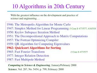
10 Algorithms in 20th Century With the greatest influence on the development and practice of science and engineering … 1946: The Metropolis Algorithm for Monte Carlo 1947: Simplex Method for Linear Programming // Com S 477/577, 418/518 1950: Krylov Subspace Iteration Method 1951: The Decompositional Approach to Matrix Computations 1957: The Fortran Optimizing Compiler 1959: QR Algorithm for Computing Eigenvalues 1962: Quicksort Algorithms for Sorting 1965: Fast Fourier Transform // Com S 477/577 1977: Integer Relation Detection 1987: Fast Multipole Method Computing in Science & Engineering, January/February 2000 Science, Vol. 287, No. 5454, p. 799, February 2000
A p q q+1 r p q q+1 r Quicksort C. A. R. Hoare 1962 Best practical sorting algorithm! p r divide conquer After partition, A[i] A[j], p i q andq+1 j r. No work is needed on combining A[p..q] and A[q+1..r]!
i i j How to Partition? pivot x 6 2 7 4 9 5 10 r j = r+1 i = p–1 p 6 2 7 4 9 5 10 x x j 5 2 7 4 9 6 10
i i j j Partitioning 5 2 7 4 9 6 10 x x A[q+1..r] A[p..q] 5 2 4 7 9 6 10 q = j i
The Procedure Partition(A, p, r) x A[p] i p – 1 j r + 1 while true do repeatj j – 1 untilA[j] x repeati i + 1 untilA[i] x ifi < j thenA[i] A[j] else returnj // different from the procedure in the textbook
The Quicksort Algorithm Quicksort(A, p, r) ifp < r thenq Partition(A, p, r) Quicksort(A, p, q) Quicksort(A, q+1, r)
2 (n ) time Performance of Quicksort Depends on how balanced the partitioning is. p = q < r Worst Case: Let n = r – p + 1 n 1 n – 1 1 n – 2 … 1 2 1 1
A Worst-Case Example The input array is already sorted. 2, 4, 5, 9, 11 2 4, 5, 9, 11 4 5, 9, 11 5 9, 11 9 11
Best Case q – p + 1 = (r – p + 1) / 2 cost n cn recursion tree n/2 n/2 cn lg n cn n/4 n/4 n/4 n/4 (n lg n)
log n 10 log n 10/9 Balanced Partitioning Suppose always a 9-to-1 proportional split. T(n) = T(9n/10) + T(n/10) + n n cn cn n/10 9n/10 cn n/100 9n/100 9n/100 81n/100 81n/1000 729n/1000 cn 1 cn T(n) = (n lg n) 1 cn
Average Case Imagine a bad split followed by a good split. n Cost of two-step partitioning: 1 n – 1 n + n – 1 = (n) (n – 1) / 2 (n – 1) / 2 similar to n Cost of one-step partitioning: n = (n) (n – 1) / 2 + 1 (n – 1) / 2 T(n) = (n lg n)
Comparison of Sorting Methods D. E. Knuth, “The Art of Computer Programming”, Vol 3, 2nd ed., p.382, 1998. Implemented on the MIX Computer. Method Space Average Max n=16 n=10000 Insertion sort n(1+) 1.25n + 13.25n 2.5n 433 1248615 2 2 Merge sort n(1+) 14.43n lnn + 4.92n 14.4n lnn 761 104716 Heapsort n 23.08n lnn + 0.01n 24.5n lnn 1068 159714 Quicksort n + 2 lgn 11.67n lnn – 1.74n 2n 470 81486 2 Median-of-3 n + 2 lgn 10.63n lnn – 2.12n n 487 74574 Quicksort 2 (Use the median of three randomly picked elements as the pivot.)
Issue with Quicksort Quicksort has the best average-case behavior. All permutations of the input sequence are assumed to be equally likely. Not necessarily true in practice! Make its behavior independent of the input ordering!
Randomization An algorithm is randomized if its behavior depends on the input random numbers No particular input causes its worst-case behavior. Choose the pivot at random! Randomized-Partition(A, p, r) i Random(p, r) A[p] A[i] return Partition(A, p, r)
r p j j j j j j j i i An Example 6 2 7 4 9 5 10 Execution 1: Random(p, r) = p + 3 4 2 7 6 9 5 10 2 4 7 6 9 5 10
j j j j j j i i i i i i i Cont’d 6 2 7 4 9 5 10 r p Execution 2: Random(p, r) = p + 2 7 2 6 4 9 5 10 5 2 6 4 9 7 10
Randomized Quicksort Randomized-Quicksort(A, p, r) ifp < r then q Randomized-Partition(A, p, r) Randomized-Quicksort(A, p, q) Randomized-Quicksort(A, q+1, r) A random sequence of good and bad choices can yield an efficient algorithm. Height of recursion tree: (lg n).
Analysis of Partitioning Assumption for simplification: All elements are distinct. x … … A: p q r After random partitioning A[k] xp k q A[k] xq+1 k r rank(x) is # elements x
Ranks and Probabilities rank(x) = 1 x p = q … … x … rank(x) 2 p q p – q + 1 = rank(x) – 1 Probability P{rank(x) = i } = 1/n, 1 i n = r – p + 1 P{q = p} = 2/n, if rank(x) = 1, 2 P{q – p + 1 = i} = 1/n, if rank(x) = i+1, i = 2, …, n–1
Average-case Running Time of Randomized-Quicksort T(n) = (1/n) (T(1) + T(n – 1) + rank(x) = 1 n – 1 (T(q) + T(n – q))) + (n) q = 1 rank(x) = q + 1 T(n) = O(n lg n) (see a separate .pdf handout) But T(n) cannot better the best case running time (n lg n) of quicksort. So T(n) = (n lg n). Running time is (n lg n)!