random va
hehe

random va
E N D
Presentation Transcript
Random Variable QUAMET1
Random Variable Definition • It is an item used to define or denote the outcomes in the sample space known as the sample points. • It assigns a numerical value to each outcome in the sample space. • It is an item whose numerical value is of a random nature, and therefore cannot be known with certainty.
Random Variable Definition • Example: If we toss a coin three times, we can use the random variable x to define the sample points of this experiment as the number of heads that occur.
Random Variable Definition • In tabular form, the probability distribution function (p.d.f.) of the random variable x is given as follows:
Random Variable Definition • In formula form:
Types of Random Variable • Discrete - this type of random variable can only assume a finite or countably infinite number of possible values. • Ex. no. of heads in a coin experiment, no. of defectives produced, demand or sales of a product in units per day, quiz average of students in Quamet1 rounded off to the nearest unit, no. of customer arrivals in a bank per hour, no. of customer complaints received per day by customer service, weight of a can of corned beef to the nearest gram, etc.
Types of Random Variable • Continuous - this type of random variable can take on any value within a given range • Ex. temperature, volume, weight, diameter, time, quiz average of a student, etc.
Types of Random Variable • Ways by which a continuous variable can be converted into a discrete variable • Specifying the level of accuracy of measurement • Ex. Continuous variable: diameter of a ball bearing in inches Discrete variable: diameter of a ball bearing to the nearest tenth of an inch • Introducing categories to describe the diff. levels of values of the random variable • Ex. Continuous variable: Final grades (raw scores) of students in Quamet1 Discrete variable: Final grades (course card grades) Grade Range Final Grade below 60 0.0 60 - 65 1.0 66 - 71 1.5 72 - 77 2.0 78 - 83 2.5 84 - 89 3.0 90 - 95 3.5 96 - 100 4.0
Probability Distribution • Probability Distribution is a table or a function which helps us determine or compute the probability associated to each value of the random variable.
Types of Probability Distribution • Discrete probability distribution - one that involves a discrete random variable. • Example: Poisson Distribution (x is the no. of arrivals per time period) • Continuous probability distribution - one that involves a continuous random variable. • Example: Exponential Distribution (t is the inter-arrival time of customers)
Discrete Probability Distribution Characteristics of a discrete probability distribution • f(x) 0 x (for all x) • f(x) = 1 • P(X = x) = f(x) refers to the value of the function when the random variable X is equal to a specific value x. • Ex. In the experiment of tossing a coin three times: P(X = 2) = f(2) = 3/8
Discrete Probability Distribution • Cumulative Distribution Function • a table or a function that determines the probability that the random variable X takes on values that are less than or equal to a specific value x • denoted by: • where: L = lower limit of possible x values
Discrete Probability Distribution • Methods of Graphing Discrete Probability Distributions • Bar Chart • Probability Histogram • Note: Area of histogram = Width x Height = Probability
Continuous Probability Distribution • The probability distribution of a continuous random variable is referred to as the continuous density function. • Note: Unlike in the discrete case, f(x) does not specify the probability that the random variable X takes on a specific value x, i.e., P(X = x) f(x). Probabilities in continuous distributions are evaluated for a given range. This time, the probability (that the random variable x takes on values within a given range x1 to x2) is represented by the area under the curve.
Continuous Probability Distribution • Derivation of the Continuous Curve • Construct histograms (as in the discrete case) • As x 0, the curve f(x) is obtained by connecting the points with a smooth curve. • Most Common Curves • Normal Curve - symmetric • Skewed to the right - positively skewed • Skewed to the left - negatively skewed
Continuous Probability Distribution • Characteristics of a continuous probability distribution 1) 2) , since Consequence: 3) 4) 5)
Continuous Probability Distribution • Cumulative Density Function • To derive the cumulative density function, just change x to t in the original probability formula. F(x) is obtained by integrating the function and then substituting t by x.
Example • The random variable x has a density function given by: f(x) = k (x+1) ; 0 x 2 = 0 ; elsewhere • Find P(0.5 x 2) • Find P(x 1.5) • Find F(x) • Use F(x) to evaluate P(x 2) and P(1 x 2.5) • Find and 2
Expectation • The expected value of the random variable x is the average of all possible values of x or the mean of the x values. It is one of the properties of a probability distribution. • Notation: E(x) or x • Note: The expectation of x is a weighted average wherein the given probabilities represent the weight.
Expectation • Example: • E(x) = 1(.5) + 2(.3) + 3(.1) + 4(.1) = 1.8 • For discrete probability distributions: • E(x) = x f(x) • For continuous probability distributions: • E(x) = x f(x) dx
Expectation of a Function • Let g(x) = pure function of the random variable x • If x is a discrete random variable, • If x is a continuous random variable,
Example • Let x = demand in units per day • Given: Selling Price (SP)=P10/unit; Variable Cost (VC)=P5/unit; Fixed Cost (FC)=P10 • Find: Expected Profit • Solution: • Profit = g(x) = 10x - 5x - 10 = 5x - 10 • Eg(x) =g(x)f(x)=(-5)(0.1) + (0)(0.3) + (5)(0.2) + (10)(0.4) = P4.5
Expectation of a Function • Decision Making Process • Decision to be made Alternatives States of Nature • States of Nature - pertains to what actually happens after a decision has been made • Note: When faced with a decision, compute the expected profit or expected cost of all the alternatives and compare. Choose the alternative that gives the greatest expected profit or least expected cost.
Variance of Random Variable (2x) • measures the dispersion or “spread” of the values of x • the average of the squares of the deviations of all the x values from the mean • just like x, 2x is a property of the probability distribution of x • Basic Formula: 2x = E(x - x)2 • Working Formula: 2x = E(x2) - (x)2 = E(x2) - E(x)2
Variance of Random Variable (2x) • Note: x and 2x are measures that provide description to a population. • Standard Deviation (x) - converts the variance into the same units as the random var. x x = (2x)1/2
Example • Given: • Req’d: 2x E(x2)=x2f(x) = (1)2(0.2) + (2)2(0.3) + (3)2(0.4) + (4)2(0.1) = 6.6 E(x) = (1)(0.2) + (2)(0.3) + (3)(0.4) + (4)(0.1) = 2.4 2x = 6.6 - (2.4)2 = 0.84 sq. units x = 0.92 units • Dispersion or spread of x values: 2.4 - 0.92 < x < 2.4 + 0.92 = 1.48 < x < 3.32
Laws of Expectation 1.) E(ax+b) = aE(x) + b • Consequently: E(ax) = aE(x) E(b) = b where a, b are constants 2.) E[g(x) h(x)] = E[g(x)] E[h(x)] • where g(x) and h(x) are 2 different functions of the random variable x
Laws of Expectation 3.) E[g(x) h(y)] = E[g(x)] E[h(y)] • where x and y are 2 different random variables 4.) E(x+y) = E(x) + E(y) 5.) E(xy) = E(x) * E(y) only if x and y are independent variables
Laws of Variance 1.) 2g(x) = E{[g(x)]2} – {E[g(x)]}2 2.) 2ax = a2 2x 3.) 2b = 0 • Consequently: 2axb = 2ax = a2 2x 4.) 2axby = a22x + b22y only if x and y are independent variables 5.) 2z = E(z2) – [E(z)]2 • where z = f(x,y) and x, y are independent variables
Joint Probability Distribution • Let x and y be two different discrete random variables. • f(x, y) – Joint Probability Distribution of x and y • probability distribution of the simultaneous occurrence of x and y; i.e., f(x, y) = P(X = x, Y = y) • gives the probability distribution that outcomes x and y can occur at the same time • For example, • Let : x - age to the nearest year of a TV set that is to be repaired y - number of defective tubes in the set • f(x, y) = f(5, 3) = probability that the TV set is 5 years old and needs 3 new tubes
Joint Probability Distribution Characteristics of a Joint Probability Distribution • f(x, y) 0 for all (x, y) • f(x, y) = 1 add up the probabilities of all possible combinations of x and y within the range • f(x, y) = P(X = x, Y = y) • For any region A in the x y plane, P [(x, y) A] = f(x, y)
Example 1 • Two refills for a ballpoint pen are selected at random from a box containing 3 blue refills, 2 red refills and 3 green refills. If X is the number of blue refills and Y is the number of red refills selected, find • the joint probability distribution function f(x, y) • P[(X, Y) A] , where A is the region {(x, y)x+y1}
Joint Density Function • Joint Density Function – joint distribution of continuous random variables Characteristics of a Joint Density Function • f(x, y) 0 • f(x, y)dxdy = 1 • P [ (X, Y) A] = f(x, y)dxdy ; for any region A in the x y plane • Note: f(x, y) - surface lying above the x y plane Probability - volume of the right cylinder bounded by the base A and the surface
Example 2 • A candy company distributes boxes of chocolates with a mixture of creams, toffees and nuts coated in both light and dark chocolate. For a randomly selected box, let X and Y, respectively be the proportion of the light and dark chocolates that are creams and suppose that the joint density function is given by: f(x, y) = k(2x + 3y) 0 x 1,0 y 1 = 0 elsewhere • Find P[(X, Y)A] where A is the region {(x, y)0<x< ½ , ¼<y<½}
Example • NOTE: • For the discrete case, P(X = x, Y = y) = f(x, y) • ex. P(x = 2, y = 1) = f(2, 1) • For the continuous case, P(X = x, Y = y) f(x, y)
Marginal Distributions • Given the joint probability distribution f(x, y) of the discrete random variable X and Y, the probability distribution g(x) of X along is obtained by summing f(x, y) over the values of y. Similarly, the probability distribution h(y) of Y alone is obtained by summing f(x, y) over the values of x. g(x) and h(y) are defined to be the marginal distributions of x and y respectively.
Marginal Distributions • For discrete case: • g(x) = f(x, y) h(y) = f(x, y) • For continuous case: • g(x) = f(x, y)dy h(y) = f(x, y) dx
Examples 3 and 4 • Derive g(x) and h(y) for Example 1. • Derive g(x) and h(y) for the joint density function in Example 2.
Conditional Distributions • Recall: Conditional Probability Formula P (B/A) = P(A B) P(A) • Consider 2 random variables X and Y: • If we let A be the event defined by X = x and B be the event that Y = y, we have, P(Y=y/X = x) = P (X = x, Y = y) P (X = x) = f(x, y) g(x) g(x) > 0 • where X and Y are discrete random variables
Conditional Distributions • P (Y=y/X=x) may actually be expressed as a probability distribution denoted by f(y/x). Therefore, f (y/x) is called by conditional distribution of the random variable Y given that X = x.
Conditional Distributions • Generalization • Let X and Y be two random variables, discrete or continuous. The conditional probability distribution of the random variable Y given that X = x, is given by f(y/x) = f(x, y) g(x) > 0 g(x) (pure function of y) • Similarly, the conditional probability distribution of the random variable X given that Y = y, is given by f (x / y) = f(x, y) h(y) > 0 h(y) (pure function of x)
Conditional Distributions • Note: f (x/y) only gives P(X=x/Y= y). If one wishes to find the probability that the discrete random variable x falls between a and b when it is known that the discrete variable Y = y, then we evaluate P (a < x < b / Y = y) = f (x / y) • Similarly, P (a < y < b / X = x) = f (x / y)
Conditional Distribution • For the continuous case: • P (a<x<b/Y= y) = f (x/y)dx • P (a<y<b/X= x) = f (y / x) dy
Example 5 • Find the conditional probability distribution of X, given that Y = 1 for Example 1 and use it to evaluate P (x=0/y=1).
Statistical Independence • Recall: P (B/A) = P(A B) P(A) P(A B) = P(A) * P (B / A) P(A B) = P(A) * P (B) • if A and B are statistically independent • Similarly, f(y/x) = f(x, y) g(x) f(x, y) = g(x) * f (y/x) f(x, y) = g(x) * h(y) • if X and Y are statistically independent
Statistical Independence • OR: f (y/x) = f(x, y) g(x) f(x, y) = g(x) * f (y / x) h(y) = f(x, y)dx = g(x) * f(y/x) dx h(y) = f (y/x) g(x) dx h(y) = f(x, y)/g(x) f(x, y) = g(x) * h(y) pure function of y if x and y are independent
Statistical Independence • Let X and Y be two random variables, discrete or continuous, with joint probability distribution f(x, y) and marginal distributions g(x) and h(y), respectively. The random variable X and Y are said to be statistically independent if and only if f(x, y) = g(x)*h(y) • for all (x, y) within their range

