Modeling the Atmospheric Transport and Deposition of Mercury to the Great Lakes

1. Modeling the Atmospheric Transport and Deposition of Mercury to the Great Lakes (work funded through the Great Lakes Restoration Initiative) Dr. Mark Cohen NOAA Air Resources Laboratory (ARL) College Park, MD, USA Briefing Slides for GLRI Monthly Call January 9, 2013

2. Atmospheric deposition is believed to be the largest • current mercury loading pathway to the Great Lakes… • How much is deposited and where does it come from? • (…this information can only be obtained via modeling...)

3. Starting Point: Where is mercury emitted to the air? 2005 Atmospheric Mercury Emissions from Large Point Sources Emissions (kg/yr) 5-10 10-50 50-100 100–300 300–500 500–1000 1000–3000 Type of Emissions Source coal-fired power plants other fuel combustion waste incineration metallurgical manufacturing & other

4. 2005 Atmospheric Mercury Emissions (Direct Anthropogenic + Re-emit + Natural) Policy-Relevant Scenario Analysis

5. HYSPLIT-Hg Lagrangian Puff Atmospheric Fate and Transport Model 0 1 2 TIME (hours) The puff’s mass, size, and location are continuously tracked… = mass of pollutant (changes due to chemical transformations and deposition that occur at each time step) Phase partitioning and chemical transformations of pollutants within the puff are estimated at each time step Initial puff location is at source, with mass depending on emissions rate Centerline of puff motion determined by wind direction and velocity Dry and wet deposition of the pollutants in the puff are estimated at each time step. deposition 2 deposition to receptor deposition 1 lake Next step: What happens to the mercury after it is emitted?

6. 2005 Atmospheric Mercury Emissions (Direct Anthropogenic + Re-emit + Natural) Policy-Relevant Scenario Analysis

7. Make sure the model is giving reasonable results Modeled vs. Measured Wet Deposition of Mercury at Sites in the Great Lakes Region

8. Keep track of the contributions from each source, and add them up Policy-Relevant Scenario Analysis Geographical Distribution of 2005 Atmospheric Mercury Deposition Contributions to Lake Erie

9. Modeling results show that these “regional” emissions are responsible for a large fraction of the modeled 2005 atmospheric deposition Results can be shown in many ways… • A tiny fraction of 2005 global mercury emissions within 500 km of Lake Erie Important policy implications!

11. Source-Attribution Results for 2005 from NOAA ARL Atmospheric Mercury Modeling, Ground-Truthed Using Atmospheric Measurements

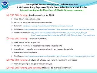
12. A multi-phase project ARL’s GLRI Atmospheric Mercury Modeling Project Jan 1, 2009 Initial Inter- and Intra-Agency Planning for FY10 GLRI Funds Jan 1, 2010 FY10 $Baseline Analysis for 2005 Jan 1, 2011 Jan 1, 2012 FY11 $Sensitivity Analysis + Extended Model Evaluation Jan 1, 2013 FY12 $ Scenario Analysis Jan 1, 2014 FY13 $ (proposed) Update Analysis (~2008) Jan 1, 2015 FY14 $ (proposed) Update Analysis (~2011) Jan 1, 2016

13. Thanks!

14. EXTRA SLIDES

17. Phase 1: Baseline Analysis for 2005 (Final Report Completed December 2011) 2005 was chosen as the analysis year, because 2005 was the latest year for which comprehensive mercury emissions inventory data were available at the start of this project Using 2005 meteorological data and emissions, the deposition and source-attribution for this deposition to each Great Lake and its watershed was estimated The model results were ground-truthed against 2005 Mercury Deposition Network data from sites in the Great Lakes region

18. Modeling Atmospheric Mercury Deposition to the Great Lakes.Final Reportfor work conducted with FY2010 funding from the Great Lakes Restoration Initiative.December 16, 2011. Mark Cohen, Roland Draxler, Richard Artz. NOAA Air Resources Laboratory,Silver Spring, MD, USA. 160 pages. http://www.arl.noaa.gov/documents/reports/GLRI_FY2010_Atmospheric_Mercury_Final_Report_2011_Dec_16.pdf http://www.arl.noaa.gov/documents/reports/Figures_Tables_GLRI_NOAA_Atmos_Mercury_Report_Dec_16_2011.pptx One-page summary: http://www.arl.noaa.gov/documents/reports/GLRI_Atmos_Mercury_Summary.pdf

19. Phase 2: Sensitivity Analysis + Extended Model Evaluation (current work, with GLRI FY11 funding) Examining the influence of uncertainties on the modeling results, by varying critical model parameters, algorithms, and inputs, and analyzing the resulting differences in results Ground-truthing the model against additional ambient monitoring data, e.g., ambient mercury air concentration measurements and wet deposition data not included in the Mercury Deposition Network (MDN)

20. Phase 3: Scenarios (next year’s work, with GLRI FY12 funding) A modeling analyses such as this is the only way to quantitatively examine the potential consequences of alternative future emissions scenarios We will work with EPA and other Great Lakes Stakeholders to identify and specify the most policy relevant scenarios to examine For each scenario, we will estimate the amount of atmospheric deposition to each of the Great Lakes and their watersheds, along with the detailed source-attribution for this deposition

21. Some Key Features of this Analysis Deposition explicitly modeled to actual lake/watershed areas • As opposed to the usual practice of ascribing portions of gridded deposition to these areas in a post-processing step

22. Some Key Features of this Analysis Deposition explicitly modeled to actual lake/watershed areas • As opposed to the usual practice of ascribing portions of gridded deposition to these areas in a post-processing step Combination of Lagrangian & Eulerian modeling • allows accurate and computationally efficient estimates of the fate and transport of atmospheric mercury over all relevant length scales – from “local” to global. • Uniquely detailed source-attribution information is created • deposition contribution to each Great Lakes and watersheds from each source in the emissions inventories used is estimated individually • The level of source discrimination is only limited by the detail in the emissions inventories • Source-type breakdowns not possible in this 1st phase for global sources, because the global emissions inventory available did not have source-type breakdowns for each grid square

23. Some Key Findings of this Analysis • “Single Source” results illustrate source-receptor relationships • For example, a “typical” coal-fired power plant near Lake Erie may contribute on the order of 100x the mercury – for the same emissions – as a comparable facility in China. Regional, national, & global mercury emissions are all important contributors to mercury deposition in the Great Lakes Basin • For Lakes Erie and Ontario, the U.S. contribution is at its most significant • For Lakes Huron and Superior, the U.S. contribution is less significant. • Local & regional sources have a much greater atmospheric deposition contributions than their emissions, as a fraction of total global mercury emissions, would suggest.

24. Some Key Findings of this Analysis (…continued) • Reasonable agreement with measurements • Despite numerous uncertainties in model input data and other modeling aspects • Comparison at sites where significant computational resources were expended – corresponding to regions that were the most important for estimating deposition to the Great Lakes and their watersheds – showed good consistency between model predictions and measured quantities. • For a smaller subset of sites generally downwind of the Great Lakes (in regions not expected to contribute most significantly to Great Lakes atmospheric deposition), less computational resources were expended, and the comparison showed moderate, but understandable, discrepancies.