Online Ascending Auctions for Gradually Expiring Items
390 likes | 570 Vues
Online Ascending Auctions for Gradually Expiring Items. Ron Lavi and Noam Nisan SISL/IST, Caltech Hebrew University. The Model (I). M identical items that “expire” at different times.

Online Ascending Auctions for Gradually Expiring Items
E N D
Presentation Transcript
Online Ascending Auctions for Gradually Expiring Items Ron Lavi and Noam NisanSISL/IST, Caltech Hebrew University
The Model (I) • M identical items that “expire” at different times. • Players arrive over time, and desire one item between their arrival time and their deadline. . . . Items: Expiration times: 1 2 3 4 Time 1 Player 1 arrival time deadline Player 2 Time 2 Player 3
The Model (II) • Player i has value vi for receiving a desired item. • Players are selfish: • All information (arrival time, deadline, value) is private, known only to the player. • Each player acts in order to maximize his own utility: value - price. • Our goal is to maximize the sum of (true) values of players that receive an item (the “social welfare”). • Applications: • In economic settings e.g. transportation tickets • In computational settings e.g. bandwidth allocation
Algorithmic Status • Well studied - equivalent to scheduling of unit jobs. • Offline optimal allocation is poly-time computable(has a matroid structure). • Lower bound of 1.618 for online approximation.[Hajek] • Online greedy is a 2 - approximation:greedy: at time t, allocate item t to the player with highest value. • This assumes obedient players that simply reveal theirprivate information.
Truthfulness and its difficulties • A popular approach: truthful auctions. • Motivating the player to reveal his true parameters. • Strong argument of dominant strategy: no matter what others do, the truth will maximize “my” utility. • Many recent positive examples for truthful auctions. • Unfortunately, we show that: Theorem: Any deterministic truthful auction for our allocation problem cannot obtain an approximation ratio better than M. • A simple truthful M - approximation exists.
How to approach this difficulty? • Relax the equilibrium notion to Bayesian - Nash: • Not a worst-case analysis. Requires strong distributional assumptions. • Add assumptions about player types. E.g. assume values in [vmin , vmax]. Then a randomized truthful 2 log(vmax - vmin) approximation exists (a special case of [BSZ]). • vs. a deterministic 2 - approximation without any assumptions when truthfulness is dropped. • Our approach: • New, relaxed, notion of equilibrium. • Worst - case analysis. No distributional assumptions. • No additional assumptions about player types.
Outline for rest of the talk • Describe two ascending auctions: • Their algorithmic properties • Intuition to an equilibrium notion that fits well • Describe a new notion of equilibrium • discuss its properties • Main theorem • Intuition for the proof
The Online Iterative Auction • Maintain temporary prices and owners for each item (initialized to 0). • At each time unit t=1,2… : • Repeat:Some player that doesn’t currently own an item temporarily takes an item, and increases the price by .Until no losing player wishes to make a new bid. • Allocate item t to its current owner for the listed price - . Keep prices and temporary owners for next time unit. • This is an adaptation of the Iterative Auction of [DGS].
Example Temp. price 0 0 =1 Temp. winner -- -- 1 2 Item Player I: v=3, d=2 Player II: v=5, d=2 Player III: v=2, d=1
Example Temp. price 1 0 =1 (phase 1) Temp. winner I -- 1 2 Item Player I: v=3, d=2 Player II: v=5, d=2 Player III: v=2, d=1
Example Temp. price 1 1 =1 (phase 2) Temp. winner I II 1 2 Item Player I: v=3, d=2 Player II: v=5, d=2 Player III: v=2, d=1
Example Temp. price 2 1 =1 (phase 3) Temp. winner III II 1 2 Item Player I: v=3, d=2 Player II: v=5, d=2 Player III: v=2, d=1
Example Temp. price 3 1 =1 (phase 4) Temp. winner I II 1 2 Item Player I: v=3, d=2 Player II: v=5, d=2 Player III: v=2, d=1
Example Temp. price 3 1 =1 (phase 4) Temp. winner I II 1 2 Item Player I: v=3, d=2 Player I did not bid for the item with lowest price. Player II: v=5, d=2 Player III: v=2, d=1
Example Temp. price 3 1 =1 Temp. winner I II 1 2 Item Result: Player I wins item 1 and pays 2. If no new player will arrive, player II will win item 2 for a price of 0. But, player II might not win at all if a new high valued player will now arrive. Player I: v=3, d=2 Player II: v=5, d=2 Player III: v=2, d=1
Players’ behaviors (the offline case) DFN([DGS]): A player is myopic if he always bids on the item with lowest price among those he desires. THM([DGS],[GS]): Assume all players arrive at time 1: • When all players are myopic then the online iterative auction finds the optimal allocation*. • When all other players are myopic, player i will maximize* his utility by behaving myopically.* up to a difference of about .
Basic structure of allocations S = the optimal allocation • A tight block B S: |B|=d and jB d(j) < d. • Tight blocks must be prefixes of S, thus contained one in the other. • Special focus in the minimal tight block f. j’ j j’’ 1 2 . . . d M
Basic structure of allocations f S = the optimal allocation • A tight block B S: |B|=d and jB d(j) < d. • Tight blocks must be prefixes of S, thus contained one in the other. • Special focus in the minimal tight block f. • Every j in f can be located first. • Therefore, its “social cost” is the value of the highest unallocated player. j’ j j’’ 1 2 . . . d M i* Highest un-allocated player determines VCG price of all players in f
The offline iterative auction with myopic players finds the optimal allocation f S = the optimal allocation • All prices in f are equal (because of the structure of swaps): • p(j’) < p(j’’) since j’ is myopic • p(j’’) < p(j’) since j’’ is myopic and has far-enough deadline. • Prices will continue to go up exactly until v(i*). j’ j j’’ 1 2 . . . d M i* Highest un-allocated player determines VCG price of all players in f
Players’ behaviors (the online case) • In the online case, non myopic behaviors might perform better. • E.g. bidding more aggressively for the current item makes sense if one anticipates that many competitive players will arrive later on. DFN: A player is semi - myopic if he bids on some item with price lower than his value. THM: If all players are semi - myopic then the online iterative auction obtains a 3 - approximation.
The Sequential Japanese Auction • Item t is sold at time t using a classic Japanese auction: • The auctioneer starts raising a price. • Each player decides whether to drop or to stay as the price ascends. • We allow to observe how many players remain at each moment. • The price halts when only one player remains. This player wins and pays the price that was reached(up to some tie breaking adjustment rule).
Example Player I: v=3, d=2 What if players I and II decide not to participate at all in the auction for item 1? Player II: v=5, d=2 Player III: v=2, d=1 Player III will win item 1. Player I will certainly not win anything. Player II might win item 2, but for a price of 3.
Example continued Player I: v=3, d=2 Suppose players I and II decide to stay until the price reaches their value, or until there remain two players in the auction (including themselves): Player II: v=5, d=2 Player III: v=2, d=1 At price=2, player III will drop. Immediately afterwards, both I and II drops. So either I or II wins and pays 2. 2 Price
Players’ behaviors (the offline case) Surprisingly, a notion of myopic behavior leads to the optimal allocation here as well: DFN: A player is myopic if, at any time t, he drops exactly: • when the price reaches his value, or • when d - t other players remain (where d is his deadline). THM: If all players arrive at time 1, and are all myopic, then the Sequential Japanese Auction finds the optimal allocation.
Proof • p*=value of highest unallocated player i*, |f|=d • Price < p* implies that no one from f drops: • At least d+1 players still remain (all f + i*) • Price is still low. • At price = p* all remaining unallocated players drop, and after them all remaining players of S. • Players of f startto drop only after all others have dropped. • winner of item 1 = optimal item 1 winner. • Continue inductively. p* Price
Players’ behaviors (the online case) • In the online case, again, bidding more aggressively for the current item makes sense if one anticipates that many competitive players will arrive later on. DFN: A player is semi - myopic if, at any time t, he drops: • not earlier than d-t other players remain, and • not later than when the price reaches his value. THM: If all players are semi - myopic then the Sequential Japanese Auction obtains a 3 - approximation.
Summary of auctions Myopic behavior Semi-myopic behavior OnlineIterative bid for the item with the lowest price bid for some item with price < value Drop when(i) price reaches value or(ii) Exactly d-t other players remain Drop in between (i) price reaches value and(ii)d-t other players remain SequentialJapanese
Proving the approximation Semi - Myopic Algorithms Lemma: Any semi - myopic algorithm obtainsa 3 - approximation. Lemma: When players are semi - myopic then both our auctions are semi - myopic algorithms. Greedy Myopic Allocate to bidder with highest value Allocate according to current best allocation Semi - myopic Allocate to someone with value > value of the winner of item t in a current best allocation ( = an optimal allocation of items t,…,M among the active players at time t ).
Set - Nash Equilibrium • The above intuition implies that we do not expect a player to follow a specific strategy. Instead, we define a set of “recommended strategies” Ri for player i. DFN: The strategy sets R1 … Rnare in Set – Nash equilibrium if a best response to every s-i R-i exists in Ri • Comment 1: If | Ri |=1, then equivalent to regular Nash. • Comment 2: Best response to mixed strategies might be outside Ri– stronger definitions can require that too. • Comment 3: Only interesting if you can say something about the outcome when everyone plays in Ri • Comment 4: Naturally generalizes to games with incomplete information without a Bayesian prior: Ri(ti)
Stronger set notions Strategies of other players R-i Player i’s strategies Ri Set domination: > (coordinate-wise)
Stronger set notions Strategies of other players R-i Player i’s strategies Ri Set mixed Nash: Eπ( ) > Eπ( )
Stronger set notions Strategies of other players R-i Player i’s strategies Ri MAX Set-Nash: MAX( ) Ri
Main Theorem: The Online Iterative Auction and the Sequential Japanese Auction Set - Nash implementa 3 - approximation of the welfare.I.e., both auctions have Set - Nash equilibrium that are all semi - myopic, hence guarantee a 3 - approximation. • All the recommended strategies are not dominated. • The recommended strategies contain best responses even if the strategies of the others are from a much larger set. • The recommended strategies do not necessarily contain b.r. to mixed recommended strategies -- We think this is an interesting open problem.
Proof structure Semi Myopic Mechanism Basic building block: Recommended Strategies thatare in Set - Nash Sequential Japanese: Online Iterative: Semi Myopic Mechanism Semi Myopic Mechanism “Ignorable extension” “Ignorable extension”
Reminder: basic structure of allocations ft St = the optimal allocation Reminder: with myopic players, the ascending auctions compute ft and VCG prices j j’ t t+1 . . . d M i* Highest un-allocated player determines VCG price of all players in ft
Semi Myopic Mechanisms Strategy space.Extended direct revelation:{ arrival time, value, “false” deadline, “true” deadline } (Similar in spirit to “2nd chance mechanisms” [NR]) Allocation rule.Compute St according to “pretend deadlines”: • Allocate item t to some player in ft . Payment Rule. • For any player i, let ct(i) be his VCG price for entering St . • Set temporary prices • The winner i pays maxt’<t pt’(i) “false” deadline If this has not passed.“true” deadline Otherwise. “pretend deadline” = ct(i)If ift.[0, ct(i) ] If i St - ft .0 Otherwise pt(i) =
Set - Nash in Semi Myopic Mechanisms Recommended strategies: declare true arrival time, value, and true “true deadline”, and any “false deadline” < true deadline. Lemma 1: When all players play recommended strategies then the allocation rule of a semi myopic mechanism is a semi myopic algorithm. Lemma 2: These recommended strategies form a Set -Nash Equilibrium.
Semi Myopic Mechanism Ascending Auctions Recommended strategies for the Online Iterative Auction:play myopically with a fake deadline until it has passed, and myopically with the real deadline afterwards. Lemma: The Semi Myopic Mechanism is embedded in the Online Iterative Auction. Proof sketch: need to show that the requirements of the semi-myopic mechanism hold: • winners belong to ft • prices are VCG Already know these from the offline analysis
Summary • We study an online setting with “gradually expiring items”. • We first saw that truthful auctions cannot perform well. • We then explored a new approach to this difficulty. • Worst case, no additional assumptions on players. • Analyzed two adaptations to classical ascending auctions. • Both obtain a 3 - approximation under a large family of selfish behaviors. • Introduced the notion of “Set - Nash equilibrium”. • Both our auctions have Set - Nash equilibrium that guarantees a 3 - approximation of the social welfare.