Presentation of Proceedings Paper
350 likes | 526 Vues
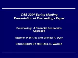
Presentation of Proceedings Paper. Application of the Option Market Paradigm to the Solution of Insurance Problems Author’s Response to Stephen Mildenhall Discussion Michael G. Wacek CAS Annual Meeting November 14, 2005. Mildenhall Criticisms.

Presentation of Proceedings Paper
E N D
Presentation Transcript
Presentation of Proceedings Paper Application of the Option Market Paradigm to the Solution of Insurance Problems Author’s Response to Stephen Mildenhall Discussion Michael G. Wacek CAS Annual Meeting November 14, 2005
Mildenhall Criticisms • Accepted paper’s main point that resemblance between call option / XL insurance concepts can lead to useful insights • Paper overstated similarity between options and insurance • In particular, paper’s assertion that “pricing math is basically the same” is “inappropriate” • Argues that insurance risks are diversified, financial risks are hedged, implying different paradigms
Wacek Mea Culpa • Mildenhall was polite • Paper overreached in claim that my formula (1.3) is a general formula for European call pricing that encompasses the Black-Scholes formula (1.1) • Author’s response shows how overarching framework is same, even if resulting formulas are different
Comparison of Formulas (1.1) and (1.3) Ct (S) = P0 ∙ N(d1) – Se-rt ∙ N(d2) (1.1) Ct (S) = e-rt (x-S) ∙ f (x) dx (1.3) (1.3) reduces to (1.1) only if underlying asset price distribution at expiry is lognormal and the expected return equals the risk free rate r N(z) is c.d.f. of standard normal; see response for d1 and d2
Parameters for Numerical Illustration of Formulas • Current stock price = $100 • Option strike (exercise) price = $100 • Time to option expiry = 20 days (20/365 years) • Stock expected return = 13% (annual, continuous) • Risk free return = 5% (annual, continuous) • Standard deviation of stock return (volatility) = 25% (annual)
Numerical Illustration of Formulas (1.1) and (1.3) • Formula (1.1) [Black Scholes]: $2.47 • Formula (1.3): $2.71 • Obviously, $2.47≠ $2.71 • Paper’s claim that (1.3) encompasses (1.1) was not “inappropriate” – it was wrong
Formula (1.3) • Formula for p.v. pure premium of aggregate excess cover • Since Black-Scholes conditions are not present, for insurance applications it is correct to use (1.3) rather than (1.1)
Pricing Paradox • If liability arises from call option on stock, use formula (1.1) • If same liability arises from aggregate excess insurance, use formula (1.3) • Why does same liability have different pricing depending on context?
Pricing Paradox Answers • Can be framed in terms of martingale measures and incomplete markets theory • Author takes more tangible approach of asset – liability matching • Within that framework the price for the transfer of a liability is function of both the liability and its optimal matching assets
Analysis of Option Liability • Assume stock price at option expiry is lognormal random variable x • Expected value of option at expiry: E(callt) = (x-S)f(x)dx = E(x) ∙ N(d1(μ))– S ∙ N(d2(μ))= P0e μ t ∙ N(d1(μ))– S ∙ N(d2(μ)) • N(z) is c.d.f of standard normal; see response for d1(μ) and d2(μ)
P0e μt ∙ N(d1(μ))– S ∙ N(d2(μ)) • First term is expected market value of the assets to be sold by option grantor to option holder at expiry • Second term is expected value of the sale proceeds from transaction
Example – Expected Option Payoff Liability • Same parameters as earlier example • 20-day option • Po = S = $100, μ = 13%, r = 5%, σ = 25% • Expected payoff = Expected market value – Expected proceeds = $56.40 - $53.68 = $2.72 • Variance = 14.45 • Standard Deviation = $3.80
Pricing of This Liability • Premium that market can be expected to ask for assuming liability depends on optimal strategy available for investment of premium to fund the liability • Assume investors / traders will find and execute optimal strategy to force asking price in market to be no greater than the level indicated by that strategy (“No arbitrage”) • Market premium = minimum expected value cost of acquiring assets to fund expected value of liability at expiry and a risk charge related to undiversifiable variability of net result • If variance can be forced to zero, risk charge is zero (B-S scenario)
Pricing This Liability in Different Available Asset Scenarios • Case A – Underlying asset is tradable • Case B – Underlying asset is not tradable • Case C – Underlying asset is not tradable, but a tradable proxy exists
Case A – Underlying Asset Tradable • Traditional actuarial approach is to invest matching assets in Treasuries • Easy to improve on that if liability arises from an option on a traded stock
Case A – Simple Hedge • At inception, buy N(d1(μ)) shares at cost of P0 ∙N(d1(μ)) • At expiry those shares expected to be worth P0 e μt ∙ N(d1(μ)) = expected liability • Expected proceeds at expiry = S ∙ N(d2(μ)) • Borrow against those proceeds at inception: Se- rt. N(d2(μ)) • Funding gap for purchase is P0 ∙ N(d1(μ)) - Se-rt ∙ N(d2(μ)) , which is amount required from option buyer (ignoring risk charge)
Case A – Simple Hedge with Numbers • Buy 0.56 shares (per option) for $56.00 • Borrow $53.54 • Charge option premium = $56.00 - $53.54 = $2.46 • Much lower than $2.71 from traditional actuarial formula (1.3) • Moreover, this asset strategy has less risk (standard deviation) than a Treasuries strategy: $1.75 vs. $3.80 • This simple hedge superior to Treasuries, but B-S found an even better one
Case A – Black-Scholes Hedge • Suppose stock trades in accordance with B-S assumptions: • Price follows geometric Brownian motion through time • Shares continuously tradable at zero transaction costs • Other • Black and Scholes showed optimal investment strategy is one of dynamic asset-liability matching conducted in continuous time
Case A – Black-Scholes Hedge • At inception, by n0 shares at cost of P0 ∙ n0,financed by a loan of L0 and call premium proceeds of P0 ∙ n0 - L0 • An instant later, adjust number of shares to n1, (to reflect any stock price change and infinitesimal passage of time) and amount of loan to L1 • If n0 and L0 have been chosen correctly and time interval is short enough, the actual gain/loss in net position (value of net stock position less value of option) is essentially zero. (Mean and variance also essentially zero) • Repeat this procedure continuously until option expires • Black and Scholes proved n0 = N(d1) and L0 = Se-rt ∙ N(d2)
Case A – Black-Scholes Hedge (continued) • Thus, call0 = P0 ∙ N(d1) – Se-rt ∙ N(d2) (1.1) • d1 = [ln(P0/S) + (r + 0.5σ2)t] / σ√t and d2 = d1 - σ√t • Since (1.1) does not depend on μ, the option seller employing this strategy not only faces no process risk but also no μ -related parameter risk
Case A – Black-Scholes Hedge with Numbers • Buy 0.5303 shares for $53.03 • Borrow $50.56 • Charge option premium = $53.03 - $50.56 = $2.47 • Compares to $2.71 and $2.46 from “actuarial” and “simple hedge” approaches • This asset strategy has no risk, so no risk charge needed
Case A - Comments • Without hedging, option seller faces expected present value liability cost of $2.71 • Market will force price of liability to $2.47 • Option seller must hedge to sell option for $2.47 without facing an expected p.v. loss of $2.71 - $2.47 = $0.24
Case A – More Comments • In practice, stocks are not continuously tradable at zero transaction costs • The less liquid the stock and the greater the trading costs the less accurate (1.1) will be in predicting the market asking price of the call option (due to residual risk and/or expenses not considered in the formula) • See Esipov & Guo (2000 Michelbacher Prizewinner)
Case B – Underlying Asset Not Tradable • Company to go public in 20 days • Assume no “when issued” or forward market for stock prior to IPO • Stock valued at $100 today • Other parameter estimates as in Case A • How to price this option?
Case B – How to Price Option? • Key question is how to invest the call premium to fund expected payoff of $2.72 • Cannot invest in underlying stock • Good strategy would seem to be to invest in Treasuries (implying formula (1.3)) • Premium = $2.71 + risk charge (standard deviation = $3.80) • μ and σ parameter risk in addition • Analogous to insurance aggregate excess scenario • Not necessarily the optimal strategy
Case C – Tradable Proxy Asset Exists • Suppose there is a similar, already public competitor to our soon-to-be-public company • Assume same return and volatility characteristics • Assume the stock price movements are believed to be correlated with r = 60%. • Possible to construct a partial hedge that results in a lower cost to fund the option liability than the Treasuries strategy
Case C – Hedge Illustration for Stock • Pursue same strategy as if hedging with actual underlying stock • Buy 0.5303 shares for $53.03 • Borrow $50.56 • Charge option premium = $53.03 - $50.56 = $2.47 + risk charge λ • Standard deviation = $3.67 vs. $3.80 for Treasuries strategy • Lower pure premium ($2.47 vs. $2.71) and lower standard deviation make this a superior strategy to investing in Treasuries
Case C – Hedge Illustration for Insurance • Suppose underlying insurance claims are 60% correlated with the consumer price index (CPI-U) • Insurer can reduce standard deviation of net result by investing in index-linked Treasury notes (TIPS) rather than conventional Treasuries • Monte Carlo analysis indicates $3.29 vs. $3.80 • P.v. pure premium = $2.71 both strategies (conventional Treasuries and TIPS)
Case C - Insurance Food for Thought • Could an insurer reduce both its risk and its required pure premium by identifying and investing in higher return securities that are partially correlated with its liabilities?
Analysis of Pricing • In all the cases A, B and C, the expected value of the option payoff (or aggregate excess liability) obligation at expiry is the same: $2.72 • Only difference are type and tradability of assets available for investment • It is the characteristics of the asset side of the asset-liability equation that determine the optimal asking price for transfer of the liability!
Analysis of Pricing (continued) • Pricing is a function of both the liability and the nature of the assets needed to fund it • In insurance applications, where there are usually no suitable assets other than Treasuries available, the liability alone appear to drive the price • However, that appears to be a special case • Actuaries should be alert to the possibility that some insurance situations might lend themselves to asset-liability matching that reduces the p.v. pure premium, risk, or both
Optimal Pricing Requires Risk Management • If the optimal asset strategy drives the pricing of the liability, it is critical that the seller actually invests according to that strategy • If option seller believes μ = 13%, and sells call option for B-S price of $2.47, it would be a mistake to invest proceeds in Treasuries • Expected result = $2.47 ert -$2.72 = -$0.24 • Standard deviation = $3.80 (vs. zero under optimal asset strategy) • Lesson: B-S assumes optimal strategy; option seller not automatically protected
Summary of Author’s Response • Author acknowledges that original claim of generality for (1.3) is wrong • However, response does show that insurance and option pricing are governed by the same overarching pricing paradigm implied by optimal asset-liability matching
Final Point on the Perils of Pricing • The dynamic asset-liability matching regimen underlying Black-Sholes formula imposes a different burden on the seller of the option than the more passive asset-liability matching seen in Case B and in insurance applications • In liquid markets, it is a mistake to sell the option for the Black-Scholes price without engaging in the optimal asset strategy • In illiquid markets, it is a mistake to sell the option for the Black-Scholes price because the optimal asset strategy does not yield that price (must use formula (1.3) instead)
Acknowledgment • Thank you to Stephen Mildenhall for his discussion