Efficient Cost Optimization in Aggregate Planning
Explore costs such as Smoothing, Holding, Shortage, Regular, Overtime, and Idle Time for effective aggregate planning. Learn how to solve planning problems using the Linear Decision Rule and understand management behavior modeling.


Efficient Cost Optimization in Aggregate Planning
E N D
Presentation Transcript
Aggregate Planning FAISAL FARIS BIN RAHIM MOHD HANEESYAH BIN CHE HASSAN NOR SYAKIRA BT ZAUKIFLI ANISAH BT ABD LATIFF
Outline • Costs in aggregate planning • Solving in aggregate planning problem • Linear decision rule (LDR) • Modeling management behavior
Costs in Aggregate Planning Smoothing Costs Holding Costs Shortage Costs Regular Costs Overtime & Subcontracting Costs Idle Time Costs
Issues in Aggregate Planning • Smoothing – refer to the cost of changing production and workforce level between periods. (Firing & Hiring Costs) • Bottleneck Problem – Inability to respond to sudden changes in demand as a result of capacity restrictions (High demand in one period & breakdown of a vital piece of equipment)
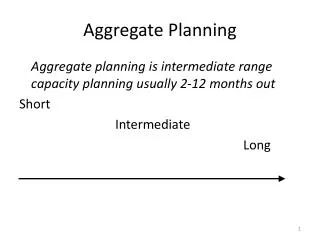
Issues in Aggregate Planning • Planning Horizon- Number of periods for which the demand forecast and aggregate planning are done. • If it is too small ( current aggregate plan may lead into not meeting the demand beyond planning horizon) • If it is too large ( forecasts into far future will be less accurate) • End-of-horizon effect
Cost in Aggregate Planning • Smoothing Cost • Hiring costs (advertising, interviewing & training) • Firing costs ( lack of labor force in future) • Assumed to be a linear function of the number of workers
Cost in Aggregate Planning Cost of Changing the Size of the Workforce • Firing costs Hiring costs
Cost in Aggregate Planning • Holding Costs • Occurs as a result of having capital tied up in inventory. • Assumed to be linear in the level of inventory • For aggregate planning, it is expressed in terms of dollars per unit held per planning period; (e.g. 100 $/month for one item)
Cost in Aggregate Planning • Shortage Costs • Shortage occurs when demands are higher than anticipated • For aggregate planning, it is assumed that excess demand is backlogged and filled in a future period. • In a highly competitive situation, the excess demand may be lost---lost sales.
Cost in Aggregate Planning • Regular Time Costs • Involve the cost of producing one unit of output during regular working hours • Overtime or Subcontracting Costs • Costs of production units not produced on regular time. • Overtime-production by regular-time employees beyond work day; • Subtracting-the production of items by an outside supplier;
Cost in Aggregate Planning • Idle Time Costs • Under utilization of workforce
PROBLEM 1 • A firm producing one product is scheduling (allocating) its January-March production capabilities. Part of the decision involves scheduling overtime work. • A unit produced on overtime costs an extra $300. Similarly, a unit made one month before it is needed incurred an inventory carrying cost of $100; two months costs $200 per unit. • The units delivered according to this schedule follows: • January - 80 units. • February - 120 units. • March - 150 units. • Production capacities are: • Formulate the production scheduling problem as a transportation problem and solve it by the Northwest Corner Rule.
PROBLEM 2 The production planner of Omega Research, a maker of industrial lenses, devised the following level output aggregate plan for the next 4 periods. Calculate the projected beginning and ending inventory for each period. Possible backorders may be shown by a negative number.
SOLUTION: Note that ending inventory = beginning inventory + planned production - demand forecast
Develop a chase demand strategy that gradually increases the inventory level to 14,000 units by the end of period 4. Show the effect of the plan on inventory level for each period. Inventory is increased by 1250 units in each period: (14,000 - 9,000)/4
Assume that the company currently has 10 employees and each employee, on average, can produce 4,000 units per period. Develop a staffing plan showing the number of employees that should be hired or laid off at the beginning period, using the following worksheet format.
FORMULA= Optimal Production Level in Period t The terms of a,b,c and d are constant that depend on the cost parameters
a) Compute the values of the aggregate production level and the number of workers that the company should be using in the current period: • Solution: Pt= 0.463(150) + 0.234(164)+ 0.111(185)+ 0.046(193)+ 0.993(180)– 0.464(45)+ 153 • Ans:……………….. W t = 0.010D t + 0.0088D t+1 + 0.0071D t+2 + 0.0054D t+2 +0.743W t-1 – 0.01I t-1 – 2.09 Ans:………………….
THE ADVANTAGES • The result is optimal production in period t will be form.
THE DRAWBACKS • The main weakness of the method is that it requires symmetric cost functions and there is no • convincing argument to justify such cost curves. • The quadratic lead to LDR there is no guarantee that the solution will be non-negative.
Modeling Management Behavior Construct model for controlling production level Created by Bowman (1963) Avoids problem arise when using traditional modeling method Exp : Avoids determine values of parameter that difficult to measure Exp : determining the accuracy of assumption that required by model.
This last method shows that the intuitive decision a good manager will take is similar to that which is provided by the linear decision rule. 1. Produce what is required However, this could result in large changes in production level and workforce. 2. Smooth production over time It could therefore be useful to introduce smoothing factor α. It is decided to select a production level P(t) which is a compromise between the current demand and the last production level.
3. Reach target inventory Introduce an additional factor β. 4. Incorporate demand forecasts Look at the future demands could avoid problems in the future The result is very similar to what the LDR proposed. The main drawback of the approach is the arbitrary character of all the choices.
D = forecast demand P = production level α = smoothing factor / exponential smoothing IN = Smoothing for inventory level β = Relative weight a = for determination of P Example Using the following values of management coefficient for Bowman smoothed production model, determine the production level should plan in the coming year with demand of 100,000 packages. Assume current production level is 150,000 packages Given : Pt-1 = 150,000 a1 = 0.3475 a2 = 0.1211 a3 = 0.556 a4 = 0.0663 a5 = 0.0023 α = 0.6 β = 0.3 IN = 40,000 Dt = 130,000 It-1 = 20,000