AGGREGATE PLANNING

1. 2 AGGREGATE PLANNING Production Planning and Control Haeryip Sihombing Fakulti Kejuruteraan PembuatanUniversiti Teknologi Malaysia Melaka

2. Chapter Outline I. Introduction II. The Concept of Aggregation III. An Overview of Production-Planning Activities IV. Framework for Aggregate Production Planning V. Techniques for Aggregate Production Planning VI. Aggregate Planning in Service Companies VII. Implementing Aggregate Production Plans - Managerial Issues VIII. Hierarchical Production Planning

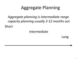
3. Aggregate production planning is medium-term capacity planning over a two to eighteen month planning horizon. It involves determining the lowest-cost method of providing the adjustable capacity for meeting production requirements.

4. Capacity Decisions Hierarchy Linkages Facilities Planning Aggregate Planning Scheduling Time Frame Facilities Planning Aggregate Planning Scheduling Time

5. Aggregation refers to the idea of focusing on overall capacity, rather than individual products or services. Aggregation is done according to: • Products • Labor • Time

6. Production Planning • Long Range Planning • Strategic planning (1-5 years) • Medium Range Planning • Employment, output, and inventory levels (2-18 months) • Short Range Planning • Job scheduling, machine loading, and job sequencing (0-2 months)

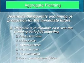
7. Aggregate production planning involves managing... • Work force levels- the number of workers required for production. • Production rates - the number of units produced per time period. • Inventory levels - the balance of unused units carried forward from the previous period.

8. Common objectives of production planning... MINIMIZE:cost, inventory levels, changes in work force levels, use of overtime, use of subcontracting, changes in production rates, changes in production rates, plant/personnel idle time MAXIMIZE:profits, customer service

9. Methods of Influencing Demand • Price Incentives • Reservations • Backlogs • Complementary Products or Services • Advertising/promotion

10. Methods of Influencing Supply • Hiring/firing workers • Overtime/slack time • Part time/temporary labor • Subcontracting • Cooperative arrangements • Inventories

11. Aggregate Production Planning Variable Costs • Hiring/firing costs • Overtime/slack time costs • Part time/temporary labor costs • Subcontracting costs • Cooperative arrangements costs • Inventory carrying costs • Backorder or stock out costs

12. Aggregate Production Planning Strategies • Chase strategy • production rates or work force levels are adjusted to match demand requirements over planning horizon • Level strategy • constant production rate or work force level is maintained over planning horizon • Mixed strategy • both inventory level changes and work force level changes occur

13. Aggregate Production Planning Techniques • Trial-and-error method • Mathematical techniques

14. Trial-and-Error Method Examples of alternative strategies: • Vary work force levels • Level work force, vary inventories and backorders • Level work force, use subcontracting • Level work force, use overtime and subcontracting

15. - Linear Decision Rule - Mgmt. Coefficient Models - Parametric Prod. Planning - Search Decision Rule - Production-Switching Heuristic - Linear Programming - Transportation Method - Goal Programming - Mixed Integer Programming - Simulation Models Mathematical Techniques

16. Managerial Issues in Aggregate Production Planning 1. APP should be tailored to the particular company and situation. 2. APP may be constrained by union contracts or company policies. 3. Mathematical techniques will likely have to be balanced with managerial judgment and experience. 4. A tendency to blur the distinction between production planning and production scheduling.

17. Aggregate Planning in Services For service companies, aggregate planning results in staffing plans that call for changing the number of employees or subcontracting.

18. The END

19. Production Planning Environment Competitor’s Behavior Raw Material Availability Market Demand Planning for Production External Capacity (outsourcing) Economic Conditions Current Physical Capacity Current Inventory Current Work Force Required Production Activities

20. Planning Production • “Long-range plan” (3-10 years) updated yearly • Inputs: aggregate forecasts (units) and current plant capacity (hours) • Decision: build new plant, expand an existing plant, create new product line, expand, contract, or delete existing product lines • Level of detail: Very Aggregated • Degree of uncertainty: High

21. Planning Production • “Intermediate-range plan” (6 month – 2 years) updated quarterly • Inputs: aggregate capacity and product decisions from the long-term plan, units are aggregated by product line or family and plant department • Decision: changes in work force, additional machines, subcontracting, overtime • Level of detail: Aggregated • Degree of uncertainty: Medium

22. Planning Production • “Short-range plan” (1 week – 6 month) updated daily or weekly • Inputs: decisions from the intermediate-term plan, units are aggregated by particular product and capacity – available hours on a particular machine, short range forecast, inventory levels, work force levels, processes • Decision: overtime and undertime, possibility of not fulfilling all demand, subcontracting, delivery dates for suppliers, product quality • Level of detail: Very Detailed • Degree of uncertainty: Low

23. Production Planning Example • Small company makes one product – plastic cases to hold CD’s. • Two different types of mold are used to produce top & bottom. • Two halves are manually put together, placed in the boxes & shipped. • The injection molding machines can make 550 pieces per hour. • A worker can finish 55 cases in 1 hour (10 workers / machine) • Forecasts of demand: 80,000 cases per month for next year  at 4 weeks/month the demand should be 20,000 cases per week. • Company runs 5 out of 7 days per week: 4,000 cases per day needed. • Each worker can not work more than 8 hours per day • 4,000/8 = 500 pieces per hour have to be produced. • Plan: 1 machine, 10 workers, 8 hours/day, 5 days/week

24. The Hierarchy of Production Planning Decisions

25. Introduction to Aggregate Planning • Goal: To plan gross work force levels and set firm-wide production plans. • Concept is predicated on the idea of an “aggregate unit” of production. May be actual units, or may be measured in weight (tons of steel), volume (gallons of gasoline), time (worker-hours), or dollars of sales. Can even be a fictitious quantity. (Refer to example in text and in slide below.)

26. Introduction to Aggregate Planning • Constant production rate can be satisfied with constant capacity. • Work force is constant, production rate slightly less that capacity of people & machines: good utilization without overloading the facilities. • Raw material usage is also constant. • If supplier and customers are also close, frequent deliveries of raw material and finished goods will keep inventory low. • How realistic is this example? • Strategies to cope with fluctuating demand? • -- change the demand -- produce at constant rate anyway • -- vary the production rate -- use combination of above strategies

27. Introduction to Aggregate Planning:Influencing Demand • Do not satisfy demand during peak periods • Capacity < Peak demand , constant production rate • Loss of some sales Japanese car manufacturers often take this stance • Determine percentage of the market share • Constant production is set at this level • Sales personal expected to sell produced amount • Ease of planning must be compared to lost revenue

28. Introduction to Aggregate Planning:Influencing Demand • Shift demand from peak periods to non-peak periods / create new demand for non-peak periods • Creating new demand can be done through advertising or incentive programs (automobile industry: rebates; telephone company’s – differential pricing system) • Smoothing demand

29. Introduction to Aggregate Planning:Influencing Demand • Produce several products with peak demand in different periods • Products should be similar, so that manufacturing them is not too different • Snowmobiles and jetskis – same engines, similar body work • Lawn-mowers – snowblowers; baseball – football equipment

30. Medium Range Planning: Aggregate Production Planning • Establish production rates by major product groups • by labor hours required or units of production • Attempt to determine monthly work force size and inventory levels that minimizes production related costs over the planning period (for 6-24 month)

31. Relevant Costs Involved • Regular time costs • Costs of producing a unit of output during regular working hours, including direct and indirect labor, material, manufacturing expenses • Overtime costs • Costs associated with using manpower beyond normal working hours • Production-rate change costs • Costs incurred in substantially altering the production rate • Inventory associated costs • Out of pocket costs associated with carrying inventory • Costs of insufficient capacity in the short run • Costs incurred as a result of backordering, lost sales revenue, loss of goodwill + costs of actions initiated to prevent shortages • Control system costs • Costs of acquiring the data for analytical decision, computational effort and implementation costs

32. Overview of the Problem Suppose that D1, D2, . . . , DT are the forecasts of demand for aggregate units over the planning horizon (T periods.) The problem is to determine both work force levels (Wt) and production levels (Pt ) to minimize total costs over the T period planning horizon.

33. Important Issues • Smoothing. Refers to the costs and disruptions that result from making changes from one period to the next. • Bottleneck Planning. Problem of meeting peak demand because of capacity restrictions. • Planning Horizon. Assumed given (T), but what is “right” value? Rolling horizons and end of horizon effect are both important issues. • Treatment of Demand. Assume demand is known. Ignores uncertainty to focus on the predictable/systematic variations in demand, such as seasonality.

34. Relevant Costs • Smoothing Costs • changing size of the work force • changing number of units produced • Holding Costs • primary component: opportunity cost of investment • Shortage Costs • Cost of demand exceeding stock on hand. Why should shortages be an issue if demand is known? • Other Costs: payroll, overtime, subcontracting.

35. Cost of Changing the Size of the Workforce

36. $ Cost Slope = Ci Slope = CP Back-orders Positive inventory Inventory Holding and Back-Order Costs

37. Aggregate Units The method is based on notion of aggregate units. They may be • Actual units of production • Weight (tons of steel) • Volume (gallons of gasoline) • Dollars (Value of sales) • Fictitious aggregate units

38. Example of fictitious aggregate units.(Example.1) One plant produced 6 models of washing machines: Model # hrs. Price % sales A 5532 4.2 285 32 K 4242 4.9 345 21 L 9898 5.1 395 17 L 3800 5.2 425 14 M 2624 5.4 525 10 M 3880 5.8 725 06 Question: How do we define an aggregate unit here?

39. Example continued • Notice: Price is not necessarily proportional to worker hours (i.e., cost): why? • One method for defining an aggregate unit: requires: .32(4.2) + .21(4.9) + . . . + .06(5.8) = 4.8644 worker hours. Forecasts for demand for aggregate units can be obtained by taking a weighted average (using the same weights) of individual item forecasts.

40. Prototype Aggregate Planning Example(this example is not in the text) The washing machine plant is interested in determining work force and production levels for the next 8 months. Forecasted demands for Jan-Aug. are: 420, 280, 460, 190, 310, 145, 110, 125. Starting inventory at the end of December is 200 and the firm would like to have 100 units on hand at the end of August. Find monthly production levels.

41. Step 1: Determine “net” demand.(subtract starting inv. from per. 1 forecast and add ending inv. to per. 8 forecast.) Month Net Predicted Cum. NetDays Demand Demand 1(Jan) 220 22022 2(Feb) 280 50016 3(Mar) 460 96023 4(Apr) 190 115020 5(May) 310 146021 6(June) 145 160517 7(July) 110 171518 8(Aug) 225 194010

43. Step 2. Graph Cumulative Net Demand to Find Plans Graphically

44. Constant Work Force Plan Suppose that we are interested in determining a production plan that doesn’t change the size of the workforce over the planning horizon. How would we do that? One method: In previous picture, draw a straight line from origin to 1940 units in month 8: The slope of the line is the number of units to produce each month.

45. Monthly Production = 1940/8 = 242.2 or rounded to 243/month. But: there are stockouts.

46. How can we have a constant work force plan with no stockouts? Answer: using the graph, find the straight line that goes through the origin and lies completely above the cumulative net demand curve:

47. From the previous graph, we see that cum. net demand curve is crossed at period 3, so that monthly production is 960/3 = 320. Ending inventory each month is found from: Month Cum. Net. Dem. Cum. Prod. Invent. 1(Jan) 220 320 100 2(Feb) 500 640 140 3(Mar) 960 960 0 4(Apr.) 1150 1280 130 5(May) 1460 1600 140 6(June) 1605 1920 315 7(July) 1715 2240 525 8(Aug) 1940 2560 620

48. But - may not be realistic for several reasons: • It may not be possible to achieve the production level of 320 unit/month with an integer number of workers • Since all months do not have the same number of workdays, a constant production level may not translate to the same number of workers each month.

49. To overcome these shortcomings: • Assume number of workdays per month is given • K factor given (or computed) where K = # of aggregate units produced by one worker in one day

50. Finding K • Suppose that we are told that over a period of 40 days, the plant had 38 workers who produced 520 units. It follows that: • K= 520/(38*40) = 0.3421 = average number of units produced by one worker in one day.