Download
1 / 26
260 likes | 443 Vues
Emerging Flux Simulations & semi-Sunspots. Bob Stein Lagerfjärd Å. Nordlund D. Georgobiani. Objectives. Complement Flux Emergence Simulations of coherent, twisted flux tubes by using minimally structured field -> horizontal, uniform, untwisted in inflows at bottom

E N D
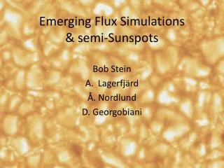
Emerging Flux Simulations& semi-Sunspots Bob Stein Lagerfjärd Å. Nordlund D. Georgobiani
Objectives • Complement Flux Emergence Simulations of coherent, twisted flux tubes by using minimally structured field -> horizontal, uniform, untwisted in inflows at bottom • Investigate formation and structure of sunspots • Provide synthetic data for validating local helioseismology and vector magnetograph inversion procedures • Investigate nature of supergranulation
Numerical Method • Spatial differencing • 6th-order finite difference • staggered (5th order interpolation) • Time advancement • 3rd order, low memory Runga-Kutta • Equation of state • tabular • including ionization, excitation • H, He + abundant elements • Radiative transfer • 3D, LTE • 4 bin multi-group opacity
Simulation set up • Vertical boundary conditions: Extrapolate lnρ; Velocity -> constant @ top, zero derivative @ bottom; energy/mass -> average value @ top, extrapolate @ bottom; • B tends to potential field @ top, • Horizontal Bx0advected into domain by inflows @bottom (20 Mm), 2 cases: Bx0 = 5 & 20kG • f-plane rotation, latitude 30 deg • Initial state – non-magnetic convection.
Flux Emergence 20 kG case, 15 – 32 hrs Average fluid rise time = 32 hrs (interval between frames =1 min) 96 km horizontal resolution -> 48 km Bv Bh
Emergent Intensity, I/<I> Flux Emergence (20 kG case) 32.1-34.2 hrs (interval between frames =1 min) Horizontal resolution 24 km.
Vertical Magnetic Field Pore/Spot Development (20 kG case) 32.1-34.2 hrs (interval between frames =1 min) Horizontal resolution 24 km.
Vertical Velocity (blue/green up, red/yellow down) & Magnetic Field lines (slice at 5 Mm) weak & horizontal B -> normal granulation vertical B -> velocity suppression weak & horizontal B -> normal granulation
Stokes Profiles Pore
I V V Q U
Magnetic Field Vertical Horizontal Active Region
Intensity Distribution Active Region Quiet Sun
Velocity Distribution Active Region
Questions: • Currently rising magnetic flux is given the same entropy as the non-magnetic plasma, so it is buoyant. What entropy does the rising magnetic flux have in the Sun? Need to compare simulations with observations for clues. • What will the long term magnetic field configuration look like? Will it form a magnetic network? Need to run for several turnover times (2 days). • What is the typical strength of the magnetic field at 20 Mm depth? Again, need to compare long runs with observations for clues. • Do we need to go to larger horizontal dimensions?
Location of Data • Slices at 1min. intervals of: Velocity & Magnetic Field, at τcont = 1, 0.1, 0.01. + Emergent Intensity, @ http://steinr.pa.msu.edu/~bob • 4 hour averages at 2 hour cadence of:sound speed, temperature, density, velocity (3 directions), magnetic field (3 components)@ steinr.pa.msu.edu/~bob/mhd48-20/AVERS4hr • Raw data cubes, averages & slices: all at http://jsoc.stanford.edu/ajax/lookdata.html (Hydro 48 Mm & 96 Mm, MHD eventually)