Download
1 / 83
830 likes | 1.02k Vues
Can computer simulations of the brain allow us to see into the mind?. Geoffrey Hinton Canadian Institute for Advanced Research & University of Toronto. Overview. Some old theories of how cortex learns and why they fail. Causal generative models and how to learn them.

E N D
Can computer simulations of the brain allow us to see into the mind? Geoffrey Hinton Canadian Institute for Advanced Research & University of Toronto
Overview • Some old theories of how cortex learns and why they fail. • Causal generative models and how to learn them. • Energy-based generative models and how to learn them.. • An example: Modeling a class of highly variable shapes by using a set of learned features. • A fast learning algorithm for deep networks that have many layers of neurons. • A really good generative model of handwritten digits. • How to see into the network’s mind.
How to make an intelligent system • The cortex has about a hundred billion neurons. • Each neuron has thousands of connections. • So all you need to do is find the right values for the weights on hundreds of thousands of billions of connections. • This task is much too difficult for evolution to solve directly. • A blind search would be much too slow. • DNA doesn’t have enough capacity to store the answer. • So evolution has found a learning algorithm and provided the right hardware environment for it to work in. • Searching the space of learning algorithms is a much better bet than searching for weights directly.
Consider a neural network with two layers of neurons. neurons in the top layer represent known shapes. neurons in the bottom layer represent pixel intensities. A pixel gets to vote if it has ink on it. Each inked pixel can vote for several different shapes. The shape that gets the most votes wins. A very simple learning task 0 1 2 3 4 5 6 7 8 9
How to learn the weights (1960’s) 1 2 3 4 5 6 7 8 9 0 The image Show the network an image and increment the weights from active pixels to the correct class. Then decrement the weights from active pixels to whatever class the network guesses.
1 2 3 4 5 6 7 8 9 0 The image Show the network an image and increment the weights from active pixels to the correct class. Then decrement the weights from active pixels to whatever class the network guesses.
1 2 3 4 5 6 7 8 9 0 The image Show the network an image and increment the weights from active pixels to the correct class. Then decrement the weights from active pixels to whatever class the network guesses.
1 2 3 4 5 6 7 8 9 0 The image Show the network an image and increment the weights from active pixels to the correct class. Then decrement the weights from active pixels to whatever class the network guesses.
1 2 3 4 5 6 7 8 9 0 The image Show the network an image and increment the weights from active pixels to the correct class. Then decrement the weights from active pixels to whatever class the network guesses.
1 2 3 4 5 6 7 8 9 0 The image Show the network an image and increment the weights from active pixels to the correct class. Then decrement the weights from active pixels to whatever class the network guesses.
The learned weights 1 2 3 4 5 6 7 8 9 0 The image Show the network an image and increment the weights from active pixels to the correct class. Then decrement the weights from active pixels to whatever class the network guesses.
A two layer network with a single winner in the top layer is equivalent to having a rigid template for each shape. The winner is the template that has the biggest overlap with the ink. The ways in which shapes vary are much too complicated to be captured by simple template matches of whole shapes. To capture all the allowable variations of a shape we need to learn the features that it is composed of. Why the simple system does not work
Good Old-Fashioned Neural Networks (1980’s) • The network is given an input vector and it must produce an output that represents: • a classification (e.g. the identity of a face) • or a prediction (e.g. the price of oil tomorrow) • The network is made of multiple layers of non-linear neurons. • Each neuron sums its weighted inputs from the layer below and non-linearly transforms this sum into an output that is sent to the layer above. • The weights are learned by looking at a big set of labeled training examples.
Good old-fashioned neural networks Compare outputs with correct answer to get error signal Back-propagate error signal to get derivatives for learning outputs hidden layers input vector
What is wrong with back-propagation? • It requires labeled training data. • Almost all data is unlabeled. • We need to fit about 10^14 connection weights in only about 10^9 seconds. • Unless the weights are highly redundant, labels cannot possibly provide enough information. • The learning time does not scale well • It is very slow in networks with more than two or three hidden layers. • The neurons need to send two different types of signal • Forward pass: signal = activity = y • Backward pass: signal = dE/dy
Overcoming the limitations of back-propagation • We need to keep the efficiency of using a gradient method for adjusting the weights, but use it for modeling the structure of the sensory input. • Adjust the weights to maximize the probability that a generative model would have produced the sensory input. This is the only place to get 10^5 bits per second. • Learn p(image) not p(label | image) • What kind of generative model could the brain be using?
The building blocks: Binary stochastic neurons • y is the probability of producing a spike. 1 0.5 synaptic weight from i to j 0 0 output of neuron i
It is easy to generate an unbiased example at the leaf nodes. It is typically hard to compute the posterior distribution over all possible configurations of hidden causes. Given samples from the posterior, it is easy to learn the local interactions 5 Sigmoid Belief Nets Hidden cause Visible effect
Explaining away • Even if two hidden causes are independent, they can become dependent when we observe an effect that they can both influence. • If we learn that there was an earthquake it reduces the probability that the house jumped because of a truck. -10 -10 truck hits house earthquake 20 20 -20 house jumps
Wake phase: Use the recognition weights to perform a bottom-up pass. Train the generative weights to reconstruct activities in each layer from the layer above. Sleep phase: Use the generative weights to generate samples from the model. Train the recognition weights to reconstruct activities in each layer from the layer below. The wake-sleep algorithm h3 h2 h1 data
How good is the wake-sleep algorithm? • It solves the problem of where to get target values for learning • The wake phase provides targets for learning the generative connections • The sleep phase provides targets for learning the recognition connections (because the network knows how the fantasy data was generated) • It only requires neurons to send one kind of signal. • It approximates the true posterior by assuming independence. • This ignores explaining away which causes problems.
Two types of generative neural network • If we connect binary stochastic neurons in a directed acyclic graph we get Sigmoid Belief Nets (Neal 1992). • If we connect binary stochastic neurons using symmetric connections we get a Boltzmann Machine (Hinton & Sejnowski, 1983)
It is not a causal generative model (like a sigmoid belief net) in which we first generate the hidden states and then generate the visible states given the hidden ones. To generate a sample from the model, we just keep stochastically updating the binary states of all the units After a while, the probability of observing any particular vector on the visible units will have reached its equilibrium value. 8 How a Boltzmann Machine models data hidden units visible units
Restricted Boltzmann Machines • We restrict the connectivity to make learning easier. • Only one layer of hidden units. • No connections between hidden units. • In an RBM, the hidden units really are conditionally independent given the visible states. It only takes one step to reach conditional equilibrium distribution when the visible units are clamped. • So we can quickly get an unbiased sample from the posterior distribution when given a data-vector : hidden j i visible
Weights Energies Probabilities • Each possible joint configuration of the visible and hidden units has an energy • The energy is determined by the weights and biases. • The energy of a joint configuration of the visible and hidden units determines its probability. • The probability of a configuration over the visible units is found by summing the probabilities of all the joint configurations that contain it.
The Energy of a joint configuration binary state of visible unit i binary state of hidden unit j biases of units i and j weight between units i and j Energy with configuration v on the visible units and h on the hidden units indexes every connected visible-hidden pair
The probability of a joint configuration over both visible and hidden units depends on the energy of that joint configuration compared with the energy of all other joint configurations. The probability of a configuration of the visible units is the sum of the probabilities of all the joint configurations that contain it. Using energies to define probabilities partition function
A picture of the maximum likelihood learning algorithm for an RBM j j j j a fantasy i i i i t = 0 t = 1 t = 2 t = infinity Start with a training vector on the visible units. Then alternate between updating all the hidden units in parallel and updating all the visible units in parallel.
16 Contrastive divergence learning: A quick way to learn an RBM j j Start with a training vector on the visible units. Update all the hidden units in parallel Update the all the visible units in parallel to get a “reconstruction”. Update the hidden units again. i i t = 0 t = 1 reconstruction data This is not following the gradient of the log likelihood. But it works well. It is approximately following the gradient of another objective function.
How to learn a set of features that are good for reconstructing images of the digit 2 50 binary feature neurons 50 binary feature neurons Decrement weights between an active pixel and an active feature Increment weights between an active pixel and an active feature 16 x 16 pixel image 16 x 16 pixel image Bartlett data (reality) reconstruction (lower energy than reality)
The weights of the 50 feature detectors We start with small random weights to break symmetry
The final 50 x 256 weights Each neuron grabs a different feature.
feature data reconstruction