Lecture: Explicit vs. Implicit - Residual, Stability, Relaxation
This lecture covers the differences between explicit and implicit methods, residual calculation in CFD, and the use of relaxation for convergence. It also discusses the solution process for advection-diffusion equations and the SIMPLE algorithm for pressure-linked equations.

Lecture: Explicit vs. Implicit - Residual, Stability, Relaxation
E N D
Presentation Transcript
Lecture Objectives: Review - Explicit vs. Implicit - Residual, Stability, Relaxation Simple algorithm
General Transport Equationunsteady-state 1-D Fully explicit method: Implicit method: Value form previous time step (known value) Make the difference between - Calculation for different time step - Calculation in iteration step
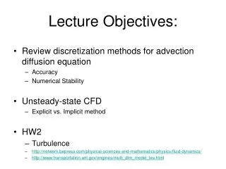
Unsteady state Advection diffusion equation, 1-D Explicit: Rarely used due to the problem with stability of calculation To achieve stable calculation Dt should be very small
Unsteady state Advection diffusion equation, 1-D Implicit: Explicit format (to solve system of equations) Iterative method: 2) Guess initial values: 3) Substitute and calculate: In iteration substitute only these values 4….) Iterate for considered time step Make the difference between iteration and calculation for next time step
Residual Example: x-exp(1/x)-2=0 Find x using iteration Explicit form 1: x=exp(1/x)+2 Explicit form 2: x=1/(ln(x-2)) Solution process: Guess x0 Iteration : x1=exp(1/x0)+2 , R1=x1-x0 X2=exp(1/x1)+2 , R2=x2-x1 …….. ……. Not all iteration process converge! See the example for the same equation
Convergence example Explicit form 2: x=1/(ln(x)-ln(2)
Residual calculation for CFD • Residual for the cell RFijk=Fkijk-Fk-1ijk • Total residual for the simulation domain RFtotal=S|RFijk| • Scaled (normalized) residual RF=S|RFijk|/FF iteration cell position Variable: p,V,T,… For all cells Flux of variable F used for normalization Vary for different CFD software
Relaxation Relaxation with iterative solvers: When the equations are nonlinear it can happen that you get divergency in iterative procedure for solving considered time step divergence variable solution convergence Solution is Under-Relaxation: Y*=f·Y(n)+(1-f)·Y(n-1) Y – considered parameter , n –iteration , f – relaxation factor For our example Y*in iteration101=f·Y(100)+(1-f) ·Y(99) f = [0-1] – under-relaxation -stabilize the iteration f = [1-2] – over-relaxation - speed-up the convergence iteration Value which is should be used for the next iteration Under-Relaxation is often required when you have nonlinear equations!
Example of relaxation Example: Advection diffusion equation, 1-D, steady-state, 4 nodes 1) Explicit format: 4 3 1 2 2) Guess initial values: 3) Substitute and calculate: Substitute and calculate: 4) Substitute and calculate: ………………………….
Navier Stokes EquationsCFD Specific Solver Continuity equation This velocities that constitute advection coefficients: F=rV Momentum x Momentum y Momentum z Pressure is in momentum equations which already has one unknown In order to use linear equation solver we need to solve two problems: • find velocities that constitute in advection coefficients 2) link pressure field with continuity equation
Pressure and velocities in NS equations How to find velocities that constitute advection coefficients? For the first step use Initial guess And for next iterative steps use the values from previous iteration
Pressure and velocities in NS equations How to link pressure field with continuity equation? SIMPLE (Semi-Implicit Method for Pressure-Linked Equations ) algorithm Dx Dx P E W Dx Ae Aw Aw=Ae=Aside We have two additional equations for y and x directions The momentum equations can be solved only when the pressure field is given or is somehow estimated. Use * for estimated pressure and the corresponding velocities
SIMPLE algorithm Guess pressure field: P*W, P*P, P*E, P*N , P*S, P*H, P*L 1) For this pressure field solve system of equations: x: ……………….. y: ……………….. z: Solution is: 2)The pressure and velocity correction P = P* + P’ P’ – pressure correction For all nodes E,W,N,S,… V = V* + V’ V’ – velocity correction Substitute P=P* + P’ and V = V* + V’ into momentum equations and obtain V’=f(P’) V = V* + f(P’) 3) Substitute V = V* + f(P’) into continuity equation solve P’ and then V 4) Solve T , k , e equations
SIMPLE algorithm start Assume V and calculate coefficients Guess p* p=p* Update V in coefficients Step1: solve V* from momentum equations Step2: introduce correction P’ and express V = V* + f(P’) Step3: substitute V into continuity equation solve P’ and then V Step4: Solve T , k , e equations no Converged (residual check) yes end
Other methods SIMPLER SIMPLEC variation of SIMPLE PISO COUPLED - use Jacobeans of nonlinear velocity functions to form linear matrix ( and avoid iteration ) V = V* + V’
HW3 Boundary condition and differencing scheme
Newton-Raphson method(example of Jacobean solver) • Faster convergence • Used in many professional tools (MathCAD, EES, MatLab, Mathematica, etc) More complex for programming • Requires linear solver Based on Taylor-Series Expansion • You need first derivative for each function to create the Jacobean matrix • Equations in the form where all side are on one side of equality sign Our simple example: X-Y/2=-1 → X-Y/2+1=0 X2-Y=-3 → X2-Y+3=0
Function values for guessed variables Jacobean matrix Unknowns (correction Dxi) Newton-Raphson method Section 6.11 of handouts Our simple example: f1 = X-Y/2+1=0 f2 = X2-Y+3=0 Steps: 0) Find derivatives d(f1)/dX =1 , d(f1)/dY =-1/2 d(f2)/dX =2X , d(f2)/dY =-1 1) Initial guess: Y(0)=2, X(0)=2 2) Find f1(Y(0),X(0))=2-2/2+1=2 f2(Y(0),X(0))=22-2+3=5 3) Using derivatives and guess values find the Jacobean matrix 4) Solve the matrix using linear solver and find DX and DY 5) Find Y(1)=Y(0)+ DY, X(1)=X(0)+ DX, Repeat step (2) with Y(1) and X(1) ….. Follow the procedure till convergence
Reynolds Averaged Navier Stokes equations Continuity: 1) Momentum: 2) 3) 4) Similar is for STy and STx 4 equations 5 unknowns → We need to model
Modeling of Turbulent Viscosity Fluid property – often called laminar viscosity Flow property – turbulent viscosity MVM: Mean velocity models TKEM: Turbulent kinetic energy equation models Additional models: LES: Large Eddy simulation models RSM: Reynolds stress models
Discretization and equation solver SIMPLE algorithm Discretization of RANS Guess p* p=p* Step1: solve V* from momentum equations Step2: introduce correction P’ and express V = V* + f(P’) Step3: substitute V into continuity equation solve P’ and then V Step4: Solve T , k , e equations no Converged (residual check) yes end
Write down this 146.6.228.78 or • 146.6.228.78 - CAEE-LicSrv07.austin.utexas.edu