Spatial Filters for Image Processing
E N D
Presentation Transcript
Image Processing Ch3: Intensity Transformation and spatial filters Part 3 Prepared by: Tahani Khatib
Ch3, lesson 6: spatial filters Spatial filters Remember that types of neighborhood: • intensity transformation: neighborhood of size 1x1 • spatial filter (or mask ,kernel, template or window): neighborhood of larger size , like 3*3 mask • The spatial filter mask is moved from point to point in an image. At each point (x,y), the response of the filter is calculated
Ch3, lesson 5: spatial filters Spatial filters
Ch3, lesson 6: Smoothing filters Spatial filters : Smoothing ( low pass) • Use:for blurring and noise reduction. • How it works?The value of every pixel is replaced by the average of the gray levels in the neighborhood. • Type of smoothing filters: • Standard average • weighted average. • 3. Median filter linear Order statistics
Ch3, lesson 6: Smoothing filters Spatial filters : Smoothinglinear smoothing : averaging kernels • Standard average weighted average. Used to reduce blurring more.
Ch3, lesson 6: Smoothing filters Spatial filters : SmoothingStandard and weighted Average- example The mask is moved from point to point in an image. At each point (x,y), the response of the filter is calculated Standard averaging filter: (110 +120+90+91+94+98+90+91+99)/9 =883/9 = 98.1 Weighted averaging filter: (110 +2 x 120+90+2 x 91+4 x 94+2 x 98+90+2 x 91+99)/16 =
Ch3, lesson 6: Smoothing filters What happens when the Values of the Kernel Fall Outside the Image??!
Ch3, lesson 6: Smoothing filters First solution :Zero padding, -ve: black border
Ch3, lesson 6: Smoothing filters border padding
Ch3, lesson 6: Smoothing filters Spatial filters : Smoothing Averaging effects: blurring + reducing noise Original image 3 x 3 averaging 5 x 5 averaging 9 x 9 averaging 15 x 15 averaging 35 x 35 averaging
Ch3, lesson 6: Smoothing filters Spatial filters : Smoothingorder statistics: Median filter becomes 95 Steps: 1. Sort the pixels in ascending order: 90,90, 91, 94, 95, 98, 99, 110, 120 2. replace the original pixel value by the median : 95
Ch3, lesson 6: Smoothing filters Spatial filters : Smoothingorder statistics: Median filter use : blurring + reduce salt and pepper noise The original image with salt and pepper noise The smoothed image using averaging The smoothed image using median
Ch3, lesson 7: sharpening filters Spatial filters : Sharpening ( high pass) • LAPLACE • SOBEL
Ch3, lesson 7: sharpening filters Spatial filters : Sharpening 1) LAPLACE Laplace kernels
Ch3, lesson 7: sharpening filters Spatial filters : Sharpening LAPLACE – 1st derivative Use: for highlighting fine detail or enhancing detail that has been blurred. Example: apply the following laplace on the highlighted pixel 154*4 – 158- 156-158-158 = -14 So the value after filter = -14 We call the resultant image: sharpened image. Filtered image=original +sharpened image The value in the filter image=154-14 =130
Ch3, lesson 7: sharpening filters Spatial filters : Sharpening LAPLACE – 1st derivative • In the sharpened image , we may get negative value, • We deal with this case in 3 ways: • Covert negative value to zero (matlab does this) • Apply 2nd derivative of laplace ( 2 ways) • Convert the negative value to the minimum value of its neighbors (after applying 1st derivative of course) • Apply laplace again to the resultant sharpened image
Ch3, lesson 7: sharpening filters Spatial filters : Sharpening LAPLACE – 2nd derivative Example: apply the following laplace 2nd derivative on the highlighted pixel 154*4 – 158- 156-158-158 = -14 Solution1: convert -14 into 1. Solution2: apply laplace to all pixels Then apply it again to our pixel:-14*4 – 10 -10 – (-6) -4 =-74 So the value after 2nd derivative filter =-74 the value of pixel in the filter image=154-74 = 80
Ch3, lesson 7: sharpening filters Spatial filters : Sharpening 1st VS 2nd derivative sharpening 1st derivative sharpening produces thicker edges in an image 1st derivative sharpening has stronger response to gray level change 2nd derivative sharpening has stronger response to fine details, such as thin lines and isolated points. 2nd derivative sharpening has double response to gray level change
Ch3, lesson 7: sharpening filters Spatial filters : Sharpening 2) Sobel Detects horizontal edges Detects vertical edges
Ch3, lesson 7: sharpening filters Spatial filters : Sharpening 2) Sobel we can apply the sobel horizontal kernel or the sobel vertical kernel or both and adding them together.
Ch3, lesson 7: sharpening filters Spatial filters : Sharpening 2) Sobel Example:
MATLAB Fspecial : for choosing the filter: X=fspecial(‘average’,[3 3]) p=fspecial(‘laplace’, 0) v=fspecial(‘sobel’) horizontal sobel Y=v’ vertical sobel Imfilter : for applying filter. m= imread(‘cameraman.tif‘); f= imfilter(m,x) this command will apply average filter on image Fp=imfilter(m,p) this command will apply laplace filter on image Imshow(fp) this command will show the laplace sharpened image imshow(m+fp) this command will show the filtered image after applying la place
MATLAB – cont. Ex. X=imtread(‘cameraman.tif‘) p=fspecial(‘laplace’, 0) Xp=imfilter(x,p, ‘replicate‘) This command will apply border padding instead of zero padding
La place filtered image La place Sharpened image
