TRAVERSING
TRAVERSING. Computations . Traversing - Computations. Traverse computations are concerned with deriving co-ordinates for the new points that were measured, along with some quantifiable measure for the accuracy of these positions.

TRAVERSING
E N D
Presentation Transcript
TRAVERSING Computations
Traversing - Computations Traverse computations are concerned with deriving co-ordinates for the new points that were measured, along with some quantifiable measure for the accuracy of these positions. The co-ordinate system most commonly used is a grid based rectangular orthogonal system of eastings (X) and northings (Y). Traverse computations are cumulative in nature, starting from a fixed point or known line, and all of the other directions or positions determined from this reference.
Traversing - Computations Angle/Bearing Computations and Balancing If angles are measured within a traverse, they need to be converted to bearings (relative to the meridian being used) in order to be used in the traverse computation. Before the bearings and azimuths are computed, the measured angles are checked for consistency and to detect any blunders.
Traversing - Computations For closed traverses, a check can be applied to ensure that the measured angles can meet the required specifications. For a closed loop traverse with n internal angles, the check that is used is: (internal angles) = (n – 2) 180 or (external angles) = (n + 2) 180 For a closed link traverse, the check is given by A1 +(angles) – A2 = (n – 1) 180 where A1 is the initial or starting azimuth, A2 is the closing or final azimuth, and n is the number of angles measured.
Traversing - Computations • The numerical difference between the computed checks and the measured sums is called the angular misclosure. There is usually a permissible or allowable limit for this misclosure, depending upon the accuracy requirements and specifications of the survey. A typical computation for the allowable misclosure is given by • = kn where n is the number of angles measured and k is a fraction based on the least division of the theodolite scale. For example, if k is 1', for a traverse with 9 measured angles, the allowable misclosure is 3 '.
Traversing - Computations Once the traverse angles are within allowable range, the remaining misclosure is distributed amongst the angles. This process is called balancing the angles : (i) arbitrary adjustment – if misclosure is small, then it may be inserted into any angle arbitrarily (usually one that may be suspect). If no angle suspect, then it can be inserted into more than one angle. (ii) average adjustment – misclosure is divided by number of angles and correction inserted into all of the angles. (most common technique) (iii) adjustment based on measuring conditions – if a line has particular obstruction that may have affected observations, misclosure may be divided and inserted into the two angles affected.
Traversing - Computations • Errors in angular measurement are not related to the size of the angle. • Once the angles have been balanced, they can be used to compute the azimuths of the lines in the traverse. • Starting from the azimuth of the original fixed control line, the internal or clockwise measured angles are used to compute the forward azimuths of the new lines. • The azimuth of this line is then used to compute the azimuth of the next line and so on.
Traversing - Computations The general formula that is used to compute the azimuths is: forward azimuth of line = back azimuth of previous line + clockwise (internal) angle The back azimuth of a line is computed from back azimuth = forward azimuth 180
Traversing - Computations Therefore for a traverse from points 1 to 2 to 3 to 4 to 5, if the angles measured at 2, 3 and 4 are 100, 210, and 190 respectively, and the azimuth of the line from 1 to 2 is given as 160, then Az23 = Az21 + angle at 2 = (160 +180) + 100 = 440 80 Az34 = Az32 + angle at 3 = (80+180) +210 = 470110 Az45 = Az43 + angle at 4 = (110+180) +190 = 480120 210 100 1 3 190 4 2 5
Traversing - Computations Once all of the azimuths have been computed, they can be checked and used for the co-ordinate computations.
Traversing - Computations B 102° 11 ' A 172° 39 ' 104° 42 ' C 118° 34 ' 113° 05 ' 352° 39 ' E D
Misclosures and Adjustments For closed traverses, since the co-ordinates of the final ending station are known, this provides a mathematical check on the computation of the co-ordinates for all of the other points. If the final computed eastings and northings are compared to the known eastings and northings for the closing station, then co-ordinate misclosures can be determined. The easting misclosure E is given by E = final computed easting – final known easting similarly, the northing misclosure N is given by N = final computed northing – final known northing
Linear Misclosure These discrepancies represent the difference on the ground between the position of the point computed from the observations and the known position of the point. The easting and northing misclosures are combined to give the linear misclosure of the traverse, where linear misclosure = (E2 + N2) N E
Traversing – Precision By itself the linear misclosure only gives a measure of how far the computed position is from the actual position (accuracy of the traverse measurements). Another parameter that is used to provide an indication of the relative accuracy of the traverse is the proportional linear misclosure. Here, the linear misclosure is divided by total distance measured, and this figure is expressed as a ratio e.g. 1 : 10000. In the example given, if the total distance measured along a traverse is 253.56m, and the linear misclosure is 0.01m, then the proportional linear misclosure is 0.01/253.56 = 1/25356 or approximately 1 : 25000
Traversing – Angular Error The required accuracy of the survey in terms of its proportional linear misclosure also defines the equipment and allowable misclosure values. For example, for a traverse with an accuracy of better than 1/5000 would require a distance measurement technique better than 1/5000, and an angular error that is consistent with this figure. If the accuracy is restricted to 1/5000, then the maximum angular error is 1/5000 = tan = 000'41" N E
Traversing – Angular Error The angular measurement for each angle should therefore be better than 000'41". The general relationship between the linear and angular error is given by the following table
Traversing – Angular Error • The maximum allowable error in the traverse which is given by • = kn k therefore depends on the maximum allowable angular error as it relates to the least count of the instrument. For a 1/5000 traverse, the value of k = 30", so = 30"n.
Traversing - Computations If a misclosure exists, then the figure computed is not mathematically closed. This can be clearly illustrated with a closed loop traverse. The co-ordinates of a traverse are therefore adjusted for the purpose of providing a mathematically closed figure while at the same time yielding the best estimates for the horizontal positions for all of the traverse stations.
Traversing - Adjustments • There are several methods that are used to adjust or balance traverses; • (i) Arbitrary method • (iii) Least-Squares • (iv) Transit rule • (v) Bowditch or Compass rule
Adjustments - Arbitrary The arbitrary method is based upon the surveyor’s individual judgement considering the measurement conditions. The Least Squares method is a rigorous technique that is founded upon probabilistic theory. It requires an over-determined solution (redundant measurements) to compute the best estimated position for each of the traverse stations.
Adjustments – Transit Rule The transit rule applies adjustments proportional to the size of the easting or northing component between two stations and the sum of the easting and northing differences. Therefore for two stations A and B, the correction to the easting and northings differences Eab and Nab are given by; correction to Eab = E(Eab/E) correction to Nab = N(Nab/N)
Adjustments – Transit Rule In this method, if a line has no easting difference, then it will not have an easting correction, and similarly, if it has no northing difference there is no northing correction. Conversely, lines with larger easting and northing differences will have larger corrections. For example, consider a traverse that has an easting misclosure E of 0.170m and a northing misclosure N of 0.361m and the easting and northing differences are 54.439m and 1.230m respectively. If the sum of the easting differences is 587.463m and the sum of the northing differences is 672.835m, then correction to Eab = 0.170(54.493/587.643) = 0.016m correction to Nab = 0.361(1.230/672.835) = 0.001m
Adjustments – Compass Rule The Bowditch or Compass rule also applies a proportional adjustment, but in this case, the distances between the stations are used in proportion to the total distance of the traverse. The corrections are given by correction to Eab = E(distanceab/total distance of traverse) correction to Nab = N(distanceab/total distance of traverse
Adjustments – Compass Rule This is the most commonly used technique for adjusting traverses. Using the above example, if the distance between A and B was 67.918m, and the total distance of the traverse was 1762.301m, then the corrections to be applied are correction to Eab = 0.170(67.918/1762.301) = 0.006m correction to Nab = 0.361(67.918/1762.301) = 0.014m
Traversing - Computations 2.1. Blunder Detection Since traverse measurements involve angular and distance measurements, it is possible for blunders to exist in the measurements that are not detected until the final co-ordinate computations are made. Angular blunders manifest themselves in the angular closure and distance blunders in the co-ordinate closure, provided that the traverse is properly closed. In both cases it is possible to localise the blunder.
Traversing - Computations To find an angular blunder, the traverse is computed without distributing the angular errors first in the forward direction, and then in the reverse direction. The point of intersection (where the co-ordinates are virtually the same) between the forward and reverse computations represents the location where the angular blunder was made, provided that only one blunder was made.
Traversing - Computations A distance blunder causes a shift in the traverse section in the direction of the incorrect length. This is detected by checking the size and direction of the linear misclosure. If the linear misclosure is near a round figure (e.g. 1m or 5m) then a blunder probably exists within the measurements. The azimuth of the misclosure is then computed by Az = tan-1(E/N)
Traversing - Computations If the azimuth is similar to any of the traverse legs, then it is likely that the distance blunder occurred when measuring this leg, and it can be corrected by remeasuring the line. If in the above example, the distance from A to B was measured as 75.11, then the resulting values for E andN would be –2.83m and –0.96m respectively. The azimuth of the misclosure would then be Az = tan-1(-2.83/-0.96) = tan-1 (2.9479) = 25115’
Traversing - Computations This azimuth is almost the same as the azimuth of the line BA, so the distance blunder has been detected in this line. This method is limited when there are several legs with nearly the same azimuth.