Circuit Analysis Tools
We will need to have our Circuit Analysis tools well in hand. We will need: Loop and Node analysis Thevenin's and Norton's Theorems Defining equations for Inductors and Capacitors RL and RC circuit analysis AC circuit analysis, phasors . Circuit Analysis Tools.

Circuit Analysis Tools
E N D
Presentation Transcript
We will need to have our Circuit Analysis tools well in hand. We will need: Loop and Node analysis Thevenin's and Norton's Theorems Defining equations for Inductors and Capacitors RL and RC circuit analysis AC circuit analysis, phasors Circuit Analysis Tools
Signals are a means of conveying information. Signals are inherently time varying quantities, since information is unpredictable, by definition. There is no such thing as a “dc signal,” or a “constant signal”, strictly speaking. Example of information: Phone conversation. Example of no information: Phone conversation between me and my grandmother. This conversation is completely predictable! Signals
Electronics is largely a way to process signals. We use voltage or current to represent signals. As the signal changes with time, so does the voltage or the current. Signals Picture taken from Hambley, 1st Edition
Signals are a means of conveying information. Signals are inherently time varying quantities, since information is unpredictable, by definition. We can have analog and digital signals. Analog signals are signals that can take on a continum of values, continuously with time. Digital signals are signals that take on discrete values, at discrete points in time. Analog and Digital Signals
Amplifiers form the basis for much of this course. It makes sense that we try to understand them. The key idea is that amplifiers give us gain. How do we get an amplifier? How do we do it? Amplifiers
Amplifiers require a new kind of component. We can use Op-Amp or transistor. We wish to consider the concept of how it works. Two key points: We amplify signals, which are time varying quantities. The amplified signals have more power. We need to get the power from somewhere. We get the power from what we call dc power supplies. Amplifiers
The reference points for voltages are usually defined, and called ground, or common. Ground is the more common term, although it may have no relationship to the potential of the earth. Below we show some common symbols for common or ground. Notation
vA, VA, va, Va– all of these refer to the voltage at point A with respect to ground. Notice that there is a polarity defined by this notation. This notation also means that we do not have to label the + and – signs on a circuit schematic to define the voltage. Once point A is labeled, the voltages vA, VA, va, and Va, are defined. Notation A + vA -
vAB, VAB, vab, Vab - refer to the voltage at point A with respect to point B . Notice that there is a polarity defined by this. This notation also means that we do not have to label the + and – signs on a circuit schematic to define the voltage. Once points A and B are labeled, the voltages vAB, VAB, vab, and Vab, are defined. Notation A + vAB - B
vA is the total instantaneous quantity (lowercaseUPPERCASE). VA is the dc component, nonvarying part of a quantity (UPPERCASEUPPERCASE). va is the ac component, varying part of a quantity (lowercaselowercase). The total instantaneous quantity is equal to the sum of the dc component and the ac component. That is, it is true that vA = VA + va. Notation A + vA -
Va is the phasor quantity (UPPERCASElowercase). (You don’t need bars.) VAA - Power supply, dc value, connected to terminal a . Note that the double subscript would otherwise have no value, since the voltage at any point with respect to that same point is zero. Generally, lowercase variables refer to quantities which can/do change, and uppercase variables to constant quantities. Va,rms refers to an rms phasor value. Notation
Voltage gain Av is the ratio of the voltage at the output to the voltage at the input. Notation
Current gain Ai is the ratio of the current at the output to the current at the input. Notation
Power gain Ap is the ratio of the power at the output to the power at the input. Notation
A dB (deciBel) is a popular, logarithmic relationship for these gains. Voltage gain in dB is 20(log10|Av|). Current gain in dB is 20(log10|Ai|). Power gain in dB is 10(log10|Ap|). Some people try to explain the factors of 10 and 20. These explanations are true, but bizarre, and somewhat beside the point. We simply need to know them. Notation
Voltage gain in dB is 20(log10|Av|). Current gain in dB is 20(log10|Ai|). Power gain in dB is 10(log10|Ap|). The key is to get these values, especially the power gain, to be greater than 1 (or 0[dB]). Thus, we move to amplifiers next. Notation
The transfer characteristic of ideal amplifier is shown by solid line. The actual amplifier start to saturate when its output, or input, exceeds a certain limit. Other forms of TC also exists. Transfer Characteristic
Amplifiers are represented in circuit models as dependent sources. There are four kinds of these, and any can be used. (Review question: Can the source transformation theorem be used with dependent sources? Ans: Yes.) Thus, there are four versions of ideal amplifier equivalent circuits. The following figures are taken from the Hambley text, Figs. 1.17, 1.28, 1.29, and 1.30. Amplifier Models
Voltage Amplifier Models This is the voltage amplifier, shown with a source and a load.
Current Amplifier Model This is the current amplifier, shown without a source and a load.
Transresistance Amplifier Model This is the transresistance amplifier, shown without a source and a load.
Transconductance Amp Model This is the transconductance amplifier, shown without a source and a load.
There are two things that always happen when you use an amplifier. 1) You have a source. 2) You have a load. The source can be represented as a Thevenin or Norton equivalent. The load can be represented as a resistance/impedance. Source and Load
With amplifiers, we call this saturation. The output voltage will not go higher than the higher power supply voltage, and will not go lower than the lower power supply voltage. A typical case is given in the following diagram, taken from the Hambley text, first edition. Amplifier Saturation
This diagram shows what happens to signals when an input which is too large is applied. In this case, the output is distorted. This form of distortion is called clipping. Amplifier Saturation
Amplifiers (Summary) General symbol of an amplifier Vin Vout Voltage gain (Av) = Vout/Vin Linear - output is proportional to input
Other types of gain and amplifiers Current amplifiers current gain (Ai) = Iout/Iin Power amplifiers power gain (Ap) = Pout/Pin
Gain in terms of decibels Typical values of voltage gain, 10, 100, 1000 depending on size of input signal Decibels often used when dealing with large ranges or multiple stages Av in decibels (dB) = 20log|Av| Ai in decibels (dB) = 20log|Ai| Ap in decibels (dB) = 10log|Ap|
Gain in terms of decibels • Av = 10 000 20log|10 000| = 80dB • Av = 1000 20log|1000| = 60dB • Av = 100 20log|100| = 40dB • Av = 10 20log|10| = 20dB • Av = -10 20log|-10| = 20dB • Av = 0.1 20log|0.1| = -20dB • Av negative - indicates a phase change (no change in dB) • dB negative - indicates signal is attenuated
Amplifier transfer characteristics Fig.1.13 An amplifier transfer characteristic that is linear except for output saturation.
Biasing an amplifier DC offset Fig.1.14(a) An amplifier transfer characteristic that shows considerable nonlinearity. (b) To obtain linear operation the amplifier is biased as shown, and the signal amplitude is kept small.
Basic characteristics of ideal amplifier For maximum voltage transfer Rout = 0 Rin = infinity