Download
1 / 14
140 likes | 299 Vues
Explore the mathematical models governing solute transport, groundwater flow, dispersion, and chemical reactions in groundwater systems. Learn about key processes like advection and dispersion, and understand the parameters and conditions influencing groundwater contamination problems.

E N D
Components of a Mathematical Model • Governing Equation • Boundary Conditions • Initial conditions (for transient problems) In full solute transport problems, we have two mathematical models: one for flow and one for transport. The governing equation for solute transport problems is the advection-dispersion equation.
Conceptual Model A descriptive representation of a groundwater system that incorporates an interpretation of the geological,hydrological, and geochemical conditions, including information about the boundaries of the problem domain.
Problem with contaminant source Contaminant source Homogeneous, isotropic aquifer Groundwater divide Groundwater divide Impermeable Rock 2D, steady state
Processes to model • Groundwater flow • Transport • Particle tracking: requires velocities and a particle tracking code. calculate path lines • (b)Full solutetransport: requires velocites and a solute transport model. calculate concentrations
v = q/n = K I / n • Processes we need to model • Groundwater flow • calculate both heads and flows (q) • Solute transport – requires information on flow (velocities) • calculate concentrations Requires a flow model and a solute transport model.
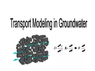
Groundwater flow is described by Darcy’s law. This type of flow is known as advection. Linear flow paths assumed in Darcy’s law True flow paths The deviation of flow paths from the linear Darcy paths is known as dispersion. Figures from Hornberger et al. (1998)
Advection-dispersion equation with chemical reaction terms. In addition to advection, we need to consider two other processes in transport problems. • Dispersion • Chemical reactions
Allows for multiple chemical species Dispersion Chemical Reactions Advection Source/sink term Change in concentration with time • is porosity; D is dispersion coefficient; v is velocity.
advection-dispersion equation groundwater flow equation
advection-dispersion equation groundwater flow equation
Flow Equation: 1D, transient flow; homogeneous, isotropic, confined aquifer; no sink/source term Transport Equation: Uniform 1D flow; longitudinal dispersion; No sink/source term; retardation
Flow Equation: 1D, transient flow; homogeneous, isotropic, confined aquifer; no sink/source term Transport Equation: Uniform 1D flow; longitudinal dispersion; No sink/source term; retardation
Models Parameters • Initial Concentration: Page 224 • Dispersion: Page 227/228