Edge detection
Understand concepts like edge detection, Laplacian operator, feature points, and good features. Learn algorithms such as Moravec, Harris detector, and Gabor functions for image matching and feature detection.


Edge detection
E N D
Presentation Transcript
Edge detection • f(x,y) viewed as a smooth function • not that simple!!! a continuous view, a discrete view, higher order lattice, … • Taylor expand in a neighborhood • f(x,y) = f(x0,y0)+ first order gradients + second-order Hessian + … • Gradients are a vector (g_x,g_y) • Hessian is a 2*2 matrix … • Local maxima/minima by first order • A scalar function of gradients, magnitude • Local maxima/minima by second order • A scalar function of Hessian, Laplacian • Difference of Gaussian as an approximation to Laplacian • Zero-crossing of DoG
is the Laplacian operator: Laplacian of Gaussian 2D edge detection filters Gaussian derivative of Gaussian filter demo
Canny Edge Operator • Smooth image I with 2D Gaussian: • Find local edge normal directions for each pixel • Compute edge magnitudes • Locate edges by finding zero-crossings along the edge normal directions (non-maximum suppression)
The edge points are thresholded local maxima after non-maximum suppression • Check if pixel is local maximum along gradient direction • requires checking interpolated pixels p and r
Original Lena Local maxima Gradient norm
From points of interest to feature points and point features! • Features • Points of interest • Feature points • Point features • Good features • Bad features
Want uniqueness Image matching! Look for image regions that are unusual • Lead to unambiguous matches in other images How to define “unusual”?
Intuition “flat” region:no change in all directions “edge”:no change along the edge direction “corner”:significant change in all directions
Moravec: points of interest • Shift in any direction would result in a significant change at a corner. Algorithm: • Shift in horizontal, vertical, and diagonal directions by one pixel. • Calculate the absolute value of the MSE for each shift. • Take the minimum as the cornerness response.
Feature detection: the math Consider shifting the window W by (u,v) • how do the pixels in W change? • compare each pixel before and after bySum of the Squared Differences (SSD) • this defines an SSD “error”E(u,v): W
Small motion assumption Taylor Series expansion of I: If the motion (u,v) is small, then first order approx is good Plugging this into the formula on the previous slide…
Feature detection: Consider shifting the window W by (u,v) • how do the pixels in W change? • compare each pixel before and after bysumming up the squared differences • this defines an “error” of E(u,v): W
This can be rewritten: For the example above • You can move the center of the green window to anywhere on the blue unit circle • Which directions will result in the largest and smallest E values? • We can find these directions by looking at the eigenvectors ofH
This can be rewritten: x- x+ Eigenvalues and eigenvectors of H • Define shifts with the smallest and largest change (E value) • x+ = direction of largest increase in E. • λ+ = amount of increase in direction x+ • x- = direction of smallest increase in E. • λ- = amount of increase in direction x-
The Harris operator Harris operator
Measure of corner response: (k – empirical constant, k = 0.04-0.06) No need to compute eigenvalues explicitly!
From points of interest to feature points and point features! • Moravaec: points of interest, in two cardinal directions • Lucas-Kanade • Tomasi-Kanade: min(lambda_1, lambda_2) > threshold • KLT tracker • Harris and Stephen (BMVC): det-k Trace^2 • Forstner in photogrammetry, from least squares matching
More unified feature detection: edges and points • f(x,y) viewed as a smooth function • Taylor expand in a neighborhood • f(x,y) = f(x0,y0)+ first order gradients + second-order Hessian + … • Gradients are a vector (g_x,g_y) • Hessian is a 2*2 matrix … • Local maxima/minima by first order • A scalar function of gradients, magnitude • Local maxima/minima by second order • A scalar function of Hessian, Laplacian • Difference of Gaussian as an approximation to Laplacian
Feature and edge detection • Convolution • Compute the gradient at each point in the image) • Nonlinear thresholding • Find points with large response (λ- > threshold) on the eigenvalues of the H matrix • Local non-maxima suppressions • Feature point • Group features • Convolution • Compute the gradient at each point in the image • Nonlinear thresholding • Find points with large response (λ- > threshold) on gradient magnitude • Local non-maxima suppressions • Edge point • Group edges
Laplacian Difference of Gaussians is an approximation to Laplacian
Motivated by matching in 3D and mosaicking • Initially proposed for correspondence matching • Proven to be the most effective in such cases according to a recent performance study by Mikolajczyk & Schmid (ICCV ’03) • Now being used for general object class recognition (e.g. 2005 Pascal challenge • Histogram of gradients • Human detection, Dalal & Triggs CVPR ’05
SIFT in one sentence is Histogram of gradients @ Harris-corner-like
The first work on local grayvalues invariants for image retrieval by Schmid and Mohr 1997, started the local features for recognition
Object Recognition from Local Scale-Invariant Features (SIFT)David G. Lowe 2004
Introduction • Image content is transformed into local feature coordinates that are invariant to translation, rotation, scale, and other imaging parameters SIFT Features
Feature Invariance • linear intensity transformation • (mild) rotation invariance by its isotropicity • scale invariance?
Scale space • Gaussian of sigma • Scale space • Intuitively coarse-to-fine • Image pyramid (wavelets) • Gaussian pyramid • Laplacian pyramid, difference of Gaussian • Laplacian is a ‘blob’ detector
Scale selection principle (Lindeberg’94) • In the absence of other evidence, assume that a scale level, at which (possibly non-linear) combination of normalized derivatives assumes a local maximum over scales, can be treated as reflecting a characteristic length of a corresponding structure in the data.
Sub-pixel localization • Sub-pixel Localization • Fit Trivariate quadratic to find sub-pixel extrema • Eliminating edges • Similar to Harris corner detector
scale • Harris-Laplacian1Find local maximum of: • Laplacian in scale • Harris corner detector in space (image coordinates) Laplacian y x Harris scale • SIFT2 Find local maximum of: • Difference of Gaussians in space and scale DoG y x DoG Different approaches 1 K.Mikolajczyk, C.Schmid. “Indexing Based on Scale Invariant Interest Points”. ICCV 20012 D.Lowe. “Distinctive Image Features from Scale-Invariant Keypoints”. IJCV 2004
Orientation • Create histogram of local gradient directions computed at selected scale • Assign canonical orientation at peak of smoothed histogram • Each key specifies stable 2D coordinates (x, y, scale, orientation)
Dominant Orientation • Assign dominant orientation as the orientation of the keypoint
Extract features • Find keypoints • Scale, Location • Orientation • Create signature • Match features • So far, we found… • where interesting things are happening • and its orientation • With the hope of • Same keypoints being found, even under some scale, rotation, illumination variation.
Creating local image descriptors • Thresholded image gradients are sampled over 16x16 array of locations in scale space • Create array of orientation histograms • 8 orientations x 4x4 histogram array = 128 dimensions
Matching as efficient nearest neigbors indexing in 128 dimensions
Comparison with HOG (Dalal ’05) • Histogram of Oriented Gradients • General object class recognition (Human) • Engineered for a different goal • Uniform sampling • Larger cell (6-8 pixels) • Fine orientation binning • 9 bins/180O vs. 8 bins/360O • Both are well engineered