Edge Detection
Edge Detection. CS485/685 Computer Vision Dr. George Bebis. Definition of Edges. Edges are significant local changes of intensity in an image. surface normal discontinuity. depth discontinuity. color discontinuity. illumination discontinuity. What Causes Intensity Changes?.

Edge Detection
E N D
Presentation Transcript
Edge Detection CS485/685 Computer Vision Dr. George Bebis
Definition of Edges • Edges are significant local changes of intensity in an image.
surface normal discontinuity depth discontinuity color discontinuity illumination discontinuity What Causes Intensity Changes? • Geometric events • surface orientation (boundary) discontinuities • depth discontinuities • color and texture discontinuities • Non-geometric events • illumination changes • specularities • shadows • inter-reflections
Goal of Edge Detection • Produce a line “drawing” of a scene from an image of that scene.
Why is Edge Detection Useful? Important features can be extracted from the edges of an image (e.g., corners, lines, curves). These features are used by higher-level computer vision algorithms (e.g., recognition).
Edge Descriptors • Edge direction:perpendicular to the direction of maximum intensity change (i.e., edge normal) • Edge strength:related to the local image contrast along the normal. • Edge position:the image position at which the edge is located.
Modeling Intensity Changes • Step edge: the image intensity abruptly changes from one value on one side of the discontinuity to a different value on the opposite side.
Modeling Intensity Changes (cont’d) • Ramp edge: a step edge where the intensity change is not instantaneous but occur over a finite distance.
Modeling Intensity Changes (cont’d) • Ridge edge: the image intensity abruptly changes value but then returns to the starting value within some short distance (i.e., usually generated by lines).
Modeling Intensity Changes (cont’d) • Roof edge: a ridge edge where the intensity change is not instantaneous but occur over a finite distance (i.e., usually generated by the intersection of two surfaces).
Main Steps in Edge Detection (1) Smoothing: suppress as much noise as possible, without destroying true edges. (2) Enhancement: apply differentiation to enhance the quality of edges (i.e., sharpening).
Main Steps in Edge Detection (cont’d) (3) Thresholding: determine which edge pixels should be discarded as noise and which should be retained (i.e., threshold edge magnitude). (4) Localization: determine the exact edge location. sub-pixelresolution might be required for some applications to estimate the location of an edge to better than the spacing between pixels.
1st derivative 2nd derivative Edge Detection Using Derivatives • Often, points that lie on an edge are detected by: (1) Detecting the local maxima or minima of the first derivative. (2) Detecting the zero-crossings of the second derivative.
Image Derivatives • How can we differentiate a digital image? • Option 1: reconstruct a continuous image, f(x,y), then compute the derivative. • Option 2: take discrete derivative (i.e., finite differences) Consider this case first!
Edge Detection Using First Derivative 1D functions (not centered at x) (centered at x) (upward) step edge ramp edge (downward) step edge roof edge
Edge Detection Using Second Derivative • Approximate finding maxima/minima of gradient magnitude by finding places where: • Can’t always find discrete pixels where the second derivative is zero – look for zero-crossing instead.
Edge Detection Using Second Derivative (cont’d) 1D functions: (centered at x+1) Replace x+1 with x (i.e., centered at x):
Edge Detection Using Second Derivative (cont’d) (upward) step edge (downward) step edge ramp edge roof edge
Edge Detection Using Second Derivative (cont’d) • Four cases of zero-crossings: {+,-}, {+,0,-},{-,+}, {-,0,+} • Slope of zero-crossing {a, -b} is: |a+b|. • To detect “strong” zero-crossing, threshold the slope.
Where is the edge?? Effect Smoothing on Derivates
Combine Smoothing with Differentiation (i.e., saves one operation)
Mathematical Interpretation of combiningsmoothing with differentiation • Numerical differentiation is an ill-posed problem. - i.e., solution does not exist or it is not unique or it does not depend continuously on initial data) • Ill-posed problems can be solved using “regularization” - i.e., impose additional constraints • Smoothing performs image interpolation.
Edge Detection Using First Derivative (Gradient) 2D functions: • The first derivate of an image can be computed using the gradient:
Gradient Representation • The gradient is a vector which has magnitude and direction: • Magnitude: indicates edge strength. • Direction: indicates edge direction. • i.e., perpendicular to edge direction (approximation) or
Approximate Gradient • Approximate gradient using finite differences:
Approximate Gradient (cont’d) • Cartesian vs pixel-coordinates: - j corresponds to x direction - i to -y direction
Approximate Gradient (cont’d) sensitive to horizontal edges! sensitive to vertical edges!
Approximating Gradient (cont’d) • We can implement and using the following masks: (x+1/2,y) good approximation at (x+1/2,y) (x,y+1/2) * * good approximation at (x,y+1/2)
Approximating Gradient (cont’d) • A different approximation of the gradient: good approximation (x+1/2,y+1/2) * • and can be implemented using the following masks:
Another Approximation • Consider the arrangement of pixels about the pixel (i, j): • The partial derivatives can be computed by: • The constant cimplies the emphasis given to pixels closer to the center of the mask. 3 x 3 neighborhood:
Prewitt Operator • Setting c = 1, we get the Prewitt operator:
Sobel Operator • Setting c = 2, we get the Sobel operator:
Edge Detection Steps Using Gradient (i.e., sqrt is costly!)
Example (using Prewitt operator) Note: in this example, the divisions by 2 and 3 in the computation of fx and fy are done for normalization purposes only
Isotropic property of gradient magnitude • The magnitude of the gradient detects edges in all directions.
Practical Issues • Noise suppression-localization tradeoff. • Smoothing depends on mask size (e.g., depends on σ for Gaussian filters). • Larger mask sizes reduce noise, but worsen localization (i.e., add uncertainty to the location of the edge) and vice versa. smaller mask larger mask
Practical Issues (cont’d) • Choice of threshold. gradient magnitude low threshold high threshold
Practical Issues (cont’d) • Edge thinning and linking.
Criteria for Optimal Edge Detection • (1) Good detection • Minimize the probability of false positives (i.e., spurious edges). • Minimize the probability of false negatives (i.e., missing real edges). • (2) Good localization • Detected edges must be as close as possible to the true edges. • (3) Single response • Minimize the number of local maxima around the true edge.
Canny edge detector • Canny has shown that the first derivative of the Gaussian closely approximates the operator that optimizes the product of signal-to-noise ratio and localization. (i.e., analysis based on "step-edges" corrupted by "Gaussian noise“) J. Canny, A Computational Approach To Edge Detection, IEEE Trans. Pattern Analysis and Machine Intelligence, 8:679-714, 1986.
Steps of Canny edge detector (cont’d) (and direction)
Canny edge detector - example original image
Canny edge detector – example (cont’d) Gradient magnitude
Canny edge detector – example (cont’d) Thresholded gradient magnitude