Edge Detection
Edge Detection. Phil Mlsna, Ph.D. Dept. of Electrical Engineering Northern Arizona University. Some Important Topics in Image Processing. Contrast enhancement Filtering (both spatial and frequency domains) Restoration Segmentation Image Compression etc. EE 460/560 course, Fall 2003


Edge Detection
E N D
Presentation Transcript
Edge Detection Phil Mlsna, Ph.D. Dept. of Electrical Engineering Northern Arizona University
Some Important Topics in Image Processing • Contrast enhancement • Filtering (both spatial and frequency domains) • Restoration • Segmentation • Image Compression etc. EE 460/560 course, Fall 2003 (formerly CSE 432/532) Edge Detection uses spatial filtering to extract important information from a scene.
Types of Edges • Physical Edges • Different objects in physical contact • Spatial change in material properties • Abrupt change in surface orientation • Image Edges • In general: Boundary between contrasting regions in image • Specifically: Abrupt local change in brightness Image edges are important clues for identifying and interpreting physical edges in the scene.
Goal: Produce an Edge Map Original Image Edge Map
Edge Detection Concepts in 1-D • Edges can be characterized as either: • local extrema of • zero-crossings of
Continuous Gradient But is a vector. We really need a scalar that gives a measure of edge “strength.” This is the gradient magnitude. It’s isotropic.
Classification of Points Let points that satisfy be edge points. PROBLEM: T Non-zero edge width Stronger gradient magnitudes produce thicker edges. To precisely locate the edge, we need to thin. Ideally, edges should be only one point thick.
Practical Gradient Algorithm • Compute for all points. • Threshold to produce candidate edge points. • Thin by testing whether each candidate edge point is a local maximum of along the direction of . Local maxima are classified as edge points.
Cameraman image Thresholded and Thinned Thresholded Gradient
Directional Edge Detection Horizontal operator (finds vertical edges) Vertical operator(finds horizontal edges) finds edges perpendicular to the direction
Directional Examples Vertical Difference Operator Horizontal Difference Operator
Discrete Gradient Operators Pixels are samples on a discrete grid. Must estimate the gradient solely from these samples. STRATEGY: Build gradient estimation filter kernels and convolve them with the image. Two basic filter concepts First difference: Central difference:
Simple Filtering Example in 1-D with Convolving [ 5 5 5 8 20 25 25 22 12 4 3 3 ] [ 0]
Simple Filtering Example in 1-D with Convolving [ 5 5 5 8 20 25 25 22 12 4 3 3 ] [ 0 0]
Simple Filtering Example in 1-D with Convolving [ 5 5 5 8 20 25 25 22 12 4 3 3 ] [ 0 0 3]
Simple Filtering Example in 1-D with Convolving [ 5 5 5 8 20 25 25 22 12 4 3 3 ] produces: [ 0 0 3 12 5 0 -3 -13 -8 -1 0 ]
Gradient Estimation 1. Create orthogonal pair of filters, 2. Convolve image with each filter: 3. Estimate the gradient magnitude:
Roberts Operator • Small kernel, relatively little computation • First difference (diagonally) • Very sensitive to noise • Origin not at kernel center • Somewhat anisotropic
Noise • Noise is always a factor in images. • Derivative operators are high-pass filters. • High-pass filters boost noise! • Effects of noise on edge detection: • False edges • Errors in edge position Key concept: Build filters to respond to edges and suppress noise.
Prewitt Operator • Larger kernel, somewhat more computation • Central difference, origin at center • Smooths (averages) along edge, less sensitive to noise • Somewhat anisotropic
Sobel Operator • 3 x 3 kernel, same computation as Prewitt • Central difference, origin at center • Better smoothing along edge, even less sensitive to noise • Still somewhat anisotropic
Discrete Operators Compared Original Roberts
Roberts Prewitt
Prewitt Sobel
T = 5 T = 10 Roberts T = 40 T = 40 T = 20
Continuous Laplacian This is a scalar. It’s also isotropic. Edge detection: Find all points for which No thinning is necessary. Tends to produce closed edge contours.
Discrete Laplacian Operators • Origin at center • Only one convolution needed, not two • Can build larger kernels by sampling Laplacian of Gaussian
Laplacian of Gaussian(Marr-Hildreth Operator) Gaussian: Let: Then:
Laplacian of Gaussian Examples s = 1.5 s = 2.0 s = 1.0
LoG Properties • One filter, one convolution needed • Zero-crossings are very sensitive to noise (2nd deriv.) • Bandpass filtering reduces noise effects • Edge map can be produced for a given scale • Scale-space or pyramid decomposition possible • Found in biological vision!! Practical LoG Filters: • Kernel at least 3 times width of main lobe, truncate • Larger kernel more computation
Summary • Edges can be detected from the derivative: • Extrema of gradient magnitude • Zero-crossings of Laplacian • Practical filter kernels; convolve with image • Noise effects • False edges • Imprecise edge locations • Correct filtering attempts to control noise • Edge map is the goal