
SDSS Analysis: Redshift, Spectra, LSS and Distributions
E N D
Presentation Transcript
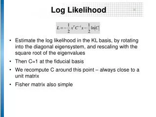
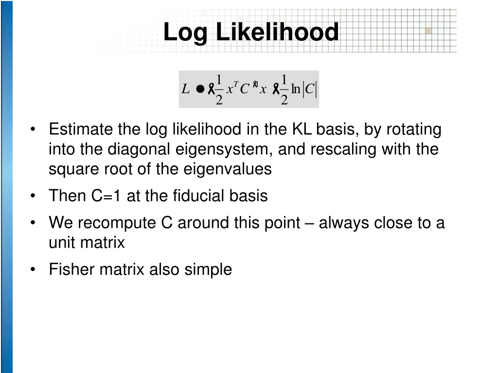
Log Likelihood • Estimate the log likelihood in the KL basis, by rotating into the diagonal eigensystem, and rescaling with the square root of the eigenvalues • Then C=1 at the fiducial basis • We recompute C around this point – always close to a unit matrix • Fisher matrix also simple
Quadratic Estimator • One can compute the correlation matrix of • P is averaged over shells, using the rotational invariance • Used widely for CMB, using the degeneracy of alm’s • Computationally simpler • But: includes 4th order contributions – more affected by nonlinearities • Parameter estimation is performed using
Distance from Redshift • Redshift measured from Doppler shift • Gives distance to zeroth order • But, galaxies are not at rest in the comoving frame: • Distortions along the radial directions • Originally homogeneous isotropic random field,now anisotropic!
Redshift Space Distortions Three different distortions • Linear infall (large scales) • Flattening of the redshift space correlations • L=2 and L=4 terms due to infall (Kaiser 86) • Thermal motion (small scales) • ‘Fingers of God’ • Cuspy exponential • Nonlinear infall (intermediate scales) • Caustics (Regos and Geller)
Power Spectrum • Linear infall is coming through the infall induced mock clustering • Velocities are tied to the density via • Using the continuity equation we get • Expanded: we get P2() and P4() terms • Fourier transforming:
r Angular Correlations • Limber’s equation
Applications • Angular clustering on small scales • Large scale clustering in redshift space
The Sloan Digital Sky Survey Special 2.5m telescope, at Apache Point, NM 3 degree field of view Zero distortion focal plane Two surveys in one Photometric survey in 5 bands detecting 300 million galaxies Spectroscopic redshift survey measuring 1 million distances Automated data reduction Over 120 man-years of development (Fermilab + collaboration scientists) Very high data volume Expect over 40 TB of raw data About 2 TB processed catalogs Data made available to the public
Current Status of SDSS • As of this moment: • About 4500 unique square degrees covered • 500,000 spectra taken (Gal+QSO+Stars) • Data Release 1 (Spring 2003) • About 2200 square degrees • About 200,000+ unique spectra • Current LSS Analyses • 2000-2500 square degrees of photometry • 140,000 redshifts
w() with Photo-z T. Budavari, A. Connolly, I. Csabai, I. Szapudi, A. Szalay, S. Dodelson,J. Frieman, R. Scranton, D. Johnston and the SDSS Collaboration • Sample selection based on rest-frame quantities • Strictly volume limited samples • Largest angular correlation study to date • Very clear detection of • Luminosity dependence • Color dependence • Results consistent with 3D clustering
ugriz L Type z Photometric Redshifts • Physical inversion of photometric measurements! Adaptive template method (Csabai etal 2001, Budavari etal 2001, Csabai etal 2002) • Covariance of parameters
343k 316k 254k 185k 280k 127k 326k 185k The Sample All: 50M mr<21 : 15M 10 stripes: 10M 0.1<z<0.3 -20 > Mr 2.2M 0.1<z<0.5 -21.4 > Mr 3.1M -20 > Mr >-21 1182k -21 > Mr >-23 931k -21 > Mr >-22 662k -22 > Mr >-23 269k
The Stripes • 10 stripes over the SDSS area, covering about 2800 square degrees • About 20% lost due to bad seeing • Masks: seeing, bright stars
The Masks • Stripe 11 + masks • Masks are derived from the database • bad seeing, bright stars, satellites, etc
The Analysis • eSpICE : I.Szapudi, S.Colombi and S.Prunet • Integrated with the database by T. Budavari • Extremely fast processing: • 1 stripe with about 1 million galaxies is processed in 3 mins • Usual figure was 10 min for 10,000 galaxies => 70 days • Each stripe processed separately for each cut • 2D angular correlation function computed • w(): average with rejection of pixels along the scan • Correlations due to flat field vector • Unavoidable for drift scan
Angular Correlations I. • Luminosity dependence: 3 cuts -20> M > -21 -21> M > -22 -22> M > -23
Angular Correlations II. • Color Dependence 4 bins by rest-frame SED type
Power-law Fits • Fitting
Bimodal w() • No change in slope with L cuts • Bimodal behavior with color cuts • Can be explained, if galaxy distribution is bimodal (early vs late) • Correlation functions different • Bright end (-20>) luminosity functions similar • Also seen in spectro sample (Glazebrook and Baldry) • In this case L cuts do not change the mix • Correlations similar • Prediction: change in slope around -18 • Color cuts would change mix • Changing slope
Redshift distribution • The distribution of the true redshift (z), given the photoz (s) • Bayes’ theorem • Given a selection window W(s) • A convolution with the selection window
Detailed modeling • Errors depend on S/N • Final dn/dz summed over bins of mr
Inversion to r0 From (dn/dz) + Limber’s equation => r0
Redshift-Space KL Adrian Pope, Takahiko Matsubara, Alex Szalay, Michael Blanton, Daniel Eisenstein, Bhuvnesh Jainand the SDSS Collaboration • Michael Blanton’s LSS sample 9s13: • SDSS main galaxy sample • -23 < Mr < -18.5, mr < 17.5 • 120k galaxy redshifts, 2k degrees2 • Three “slice-like” regions: • North Equatorial • South Equatorial • North High Latitude
Pixelization • Originally: 3 regions • North equator: 5174 cells, 1100 modes • North off equator: 3755 cells, 750 modes • South: 3563 cells, 1300 modes • Likelihoods calculated separately, then combined • Most recently: 15K cells, 3500 modes • Efficiency • sphere radius = 6 Mpc/h • 150 Mpc/h < d < 485 Mpc/h (80%): 95k • Removing fragmented patches: 70k • Keep only cells with filling factor >74%: 50k
Redshift Space Distortions • Expand correlation function • cnL = Skfk(geometry)b k • b = W0.6/b redshift distortion • b is the bias • Closed form for complicated anisotropy=> computationally fast
Wb/Wm Shape Wmh = 0.25 ± 0.04 fb = 0.26 ± 0.06 Wmh
b s8 Both depend on b b = 0.40 ± 0.08 s8 = 0.98 ± 0.03
Parameter Estimates • Values and STATISTICAL errors: Wh = 0.25 ± 0.05 Wb/Wm= 0.26 ± 0.06 b = 0.40 ± 0.05 s8 = 0.98 ± 0.03 • 1s error bars overlap with 2dF Wh = 0.20 ± 0.03 Wb/Wm = 0.15 ± 0.07 With h=0.71 Wm = 0.35 b = 1.33 s8m = 0.73 Degeneracy: Wh = 0.19 Wb/Wm= 0.17 also within 1s With h=0.7 Wm = 0.27 b = 1.13 s8m = 0.86 WMAP s8m = 0.84
Technical Challenges • Large linear algebra systems • KL basis: eigensystem of 15k x 15k matrix • Likelihood: inversions of 5k x 5k matrix • Hardware / Software • 64 bit Intel Itanium processors (4) • 28 GB main memory • Intel accelerated, multi-threaded LAPACK • Optimizations • Integrals: lookup tables, symmetries, 1D numerical • Minimization techniques for likelihoods
Systematic Errors • Main uncertainty: • Effects of zero points, flat field vectors result in large scale, correlated patterns • Two tasks: • Estimate how large is the effect • De-sensitize statistics • Monte-Carlo simulations: • 100 million random points, assigned to stripes, runs, camcols, fields, x,y positions and redshifts => database • Build MC error matrix due to zeropoint errors • Include error matrix in the KL basis • Some modes sensitive to zero points (# of free pmts) • Eliminate those modes from the analysis => projectionStatistics insensitive to zero points afterwards
SDSS LRG Sample • Three redshift samples in SDSS • Main Galaxies • 900K galaxies, high sampling density, but not very deep • Luminous Red Galaxies • 100K galaxies, color and flux selected • mr < 19.5, 0.15 < z < 0.45, close to volume-limited • Quasars • 20K QSOs, cover huge volume, but too sparsely sampled • LRGs on a “sweet spot” for cosmological parameters: • Better than main galaxies or QSOs for most parameters • Lower sampling rate than main galaxies, but much more volume (>2 Gpc3) • Good balance of volume and sampling
LRG Correlation Matrix • Curvature cannot be neglected • Distorted due to the angular-diameter distance relation (Alcock-Paczynski) including a volume change • We can still use a spherical cell, but need a weighting • All reduced to series expansions and lookup tables • Can fit for WL or w! • Full SDSS => good constraints • b and s8 no longer a constant b = b(z) = W(z)0.6 / b(z) • Must fit with parameterized bias model, cannot factor correlation matrix same way (non-linear)
Fisher Matrix Estimators • SDSS LRG sample • Can measureWLto ± 0.05 • Equation of state:w = w0 + z w1 Matsubara & Szalay (2002)
Summary • Large samples, selected on rest-frame criteria • Excellent agreement between redshift surveysand photo-z samples • Global shape of power spectrum understood • Good agreement with CMB estimations • Challenges: • Baryon bumps, cosmological constant, equation of state • Possible by redshift surveys alone! • Even better by combining analyses! • We are finally tying together CMB and low-z