Download

1 / 22
230 likes | 445 Vues
Convolution and the Fast Fourier Transform. Tarik Guelzim. Vectors. Given two vectors a=(a 0 ,a 1 ,...,a n-1 ) b=(b 0 ,b 1 ,...,b n-1 ) we can compute the sum a+b or the inner product, producing a.b we can also produce the convolution a*b. Convolution.

E N D
Convolution and the Fast Fourier Transform Tarik Guelzim
Vectors • Given two vectors • a=(a0,a1,...,an-1) • b=(b0,b1,...,bn-1) • we can compute the sum a+b • or the inner product, producing a.b • we can also produce the convolution a*b
Convolution • The convolution of two vectors of length n is a vector with 2n-1 coordinates where: aibi (i,j):i+j=k i,j<n In other words, a*b = (a0b0, a0b1 + a1b0, a0b2+a1b1+a2b0,...,an-2bn-1+ an-2bn-2,an-1bn-1).
Simply speaking ... • This definition is simply: a0b0 a1b0 a2b0 ... an-1b0 a0b1 a1b1 a2b1 ... an-1b1 a0bn-1 a1bn-1 a2bn-1 ... an-1bn-1 ... ... ... ... we compute the coordinates in the convolution vector by summing along the diagonals.
simply it is ... • This definition is simply: a0b2 a0bn-1 a1bn-1 a2bn-1 ... an-1bn-1 a0b0 a1b0 a2b0 ... an-1b0 a0b1 a1b1 a2b1 ... an-1b1 ... ... ... ... a*b = (a0b0, a0b1 + a1b0, a0b2+a1b1+a2b0,...,an-2bn-1+ an-2bn-2,an-1bn-1).
Polynomial Multiplication • A(x) = a0 + a1x + a2x2 + ... + am-1xm-1 • B(x) =b0+b1x + b2x2 + ... + bm-1xm-1 • we can represent them by vector coefficients where: • a = (a0,a1,.., am-1) and b = (b0,b1,.., bm-1) • so now given A(x) and B(x) consider C(x) such that C(x) = A(x)B(x) • the coefficients of C(x) are c = (c0,c1,.., c2n-2) • we can compute the coef. of xk Ck = aibj (i,j):i+j=k
Example • A(x) = 1 + 2x + 3x2 and B(x) = 2 + 3x +4x2 • A = (1, 2, 3) and B = (2, 3, 4) 1*2 2*2 3*2 2 3 4 4 6 8 6 9 12 1*3 2*3 3*3 1*4 2*4 3*4 = A(x) * B(x) = 2+7+16x2+17x3+12x4 C = (2, 7,16,17,12)
Computing the convolution • Computing the convolution with this method takes O(n2) because for every pair (i,j) we calculate the product aibi • Can we do better that this quadratic running time?
Algorithm design • Again suppose we are given two vectors: • a = (a0,a1,.., am-1) and b = (b0,b1,.., bm-1) • what we want is to compute the product of C(x) = A(x)B(x) in O(n log n). • once done, we can read off the desired answer directly from the coef. of C(x).
Rather that multiplying A and B symbolically we treat them as functions of x. • step 1: we choose 2n values (C has 2n-1 coordinates) x1,x2,...,x2n and evaluate A(xj) and b(xj) for each j = 1, 2,...,2n • step 2: we compute C(Xj)simply by A(xj)*b(xj) • step 3: we can recover C from its values on x1, x2, ..,x2n by using polynomial interpolation.
Polynomial interpolation • any polynomial of degree d can be reconstructed from its values on any set of d+1 or more points. • we can observe that since A and B each have a degree at most n-1, the product C has degree at most 2n-2 • [a(x) = 0+0x+x2 and b(x) = 0+0x+x2 • a*b = x4 ]
The problem is ... • step 1: we choose 2n values (C has 2n-1 coordinates) x1,x2,...,x2n and evaluate A(xj) and b(xj) for each j = 1, 2,...,2n • step 2: we compute C(Xj)simply by A(xj)*b(xj) O(n) • step 3: we can recover C from its values on x1, x2, ..,x2n by using polynomial interpolation. since we are trying to perform 2n evaluations we fall back into O(n2) again
The Trick • the idea is to find a set of 2n values x1,x2,...,x2n that are intimately related in some way such that the work in evaluating A and B on all of them can be shared across different evaluations.
Complex Roots of Unity • recall that a complex number x+yi can also be written in polar coordinate as: reφi • where eπi = -1 and e2πi = 1 • for a positive integer k, the polynomial equation xk = 1 has k distinct complex roots and they are • ωj,k= e2πji/k ( for j = 0,1,2,...,k-1) • (e2πji/k )k = e2πji = (e2πi)j = 1j = 1 • each of these numbers is distinct, so they are all of the roots.
The representation of polynomial P by its values on the (d +1)st roots of unity is referred to as the discrete Fourier transform (DFT).
Polynomial Evaluation • our goal is to design an algorithm that evaluates A on each of the (2n)th roots of unity recursively. • we need to satisfy the recurrence relation 2T(n/2)+O(n).
Divide and Conquer • we need to define two polynomials Aeven and Aodd • Aeven(x)=a0+a2x+a4x2+...+an-2x(n-2)/2 • Aodd(x)=a1+a3x+a5x2+...+an-1x(n-1)/2 • A(x) = Aeven(x2)+xAodd(x2) • Aeven and Aodd both have half the input and only n roots of unity to evaluate so the total time is • 2T(n/2)
To satisfy the recurrence relation we need to evaluate A(x) = Aeven(x2)+xAodd(x2) in O(n). • given ωj,2n= e2πji/2n the quantity ω2j,2n= (e2πji/2n )2 = e2πji/n and this is an nth root of unity so when we try to compute A(x) = Aeven(x2)+ xAodd(x2) the right side has already been performed in a recursive step. • thus, A(x) for 2n can be done in O(n). with this we satisfied the O(n log n) bound.
Reconstructing C • we can do the same to evaluate B on the (2n)th roots of unity and to compute C(ωj,n) = A(ωj,2n)B(ωj,2n) • consider a polynomial : • c(x) = Σ • we want to reconstruct it from its values C(ωj,2n) • we need to define D(x) = Σ 2n-1 csxs s=0 2n-1 dsxs s=0 Where ds = C(ωj,2n)
Theorem 2n-1 csxs For any polynomial • c(x) = Σ s=0 2n-1 • D(ωj,2n) = Σ C(ωs,2n) xs s=0 we have that Cs = 1/2n D(ω2n-s, 2n) After evaluating the polynomial D(x) at the (2n)th roots of unity give us the coefficient of the polynomial C(x) in reverse order All the evaluation of D can be done in O (n log n) using the same divide and conquer approach we showed previously.
What we proved is ... • Using the FFT to determine the product polynomial C(x), we can compute the convolution of the original vectors a and b in o(n log n) instead of O(n2)
Applications of Convolution • Combining histograms is one application of Convolution. • For example if we have two histograms of men and women and their salaries and we want to get another histogram from the previous to of all pairs (man,woman) that have a combined income of k we in a sense add all the terms i+j=k. • Most of the applications of convolution are in the signal processing domain where it is used to convert data from the time domain to the frequency domain.