Fast Fourier Transform
Fast Fourier Transform. 向 华 武汉大学数学与统计学院. Fast Fourier Transform. The Fast Fourier Transform (FFT) is a very efficient algorithm for performing a discrete Fourier transform


Fast Fourier Transform
E N D
Presentation Transcript
Fast Fourier Transform 向 华 武汉大学数学与统计学院
Fast Fourier Transform • The Fast Fourier Transform (FFT) is a very efficient algorithm for performing a discrete Fourier transform • A.C.Clairaut,cosine-only finite Fourier series(1754),J.L.Lagrange,sine-only series(1762),Bernoulli,a series of sine and cosine.FFT principle first used by Gauss in 1805? • FFT algorithm published by Cooley & Tukey in 1965 • In 1969, the 2048 point analysis of a seismic trace took 13 ½ hours. Using the FFT, the same task on the same machine took 2.4 seconds!
Fourier 变换: 存在的条件: Jean Baptiste Joseph Fourier (1768 - 1830) 反变换: 注意不同文献中的定义,特别是系数 ,exp(-i2πkx)…
1 d(t) w t delta 函数 TopHat 函数
cos(w0t) w t +w0 -w0 0 0 cosine 函数 sine 函数
位移性质: 相似性质: -a a
energy theorem, Rayleigh’s theorem The zero frequency point 反变换: 代入
常用的其他定义 连续傅立叶变换 (Continuous Fourier Transform) 离散傅立叶变换 (Discrete Fourier Transform) 连续傅立叶变换(Continuous Fourier Transform) where 离散傅立叶变换(Discrete Fourier Transform) For u=0,1,2,…,N-1 For x=0,1,2,…,N-1
连续Fourier变换(Continuous Fourier Transform) 反变换 DFT: IDFT:
omega = exp(-2*pi*i/n); j = 0:n-1; k = j'; F = omega.^(k*j); % an easier,and quicker, way to generate F is F = fft(eye(n));
离散Fourier变换(DFT) (此处定义与教材和MATLAB保持一致) Requires N2 complex multiplies and N(N-1) complex additions WN=e-i 2π/N 对称性: 周期性:
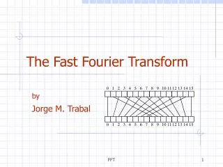
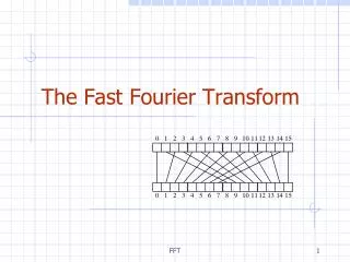
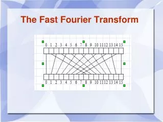
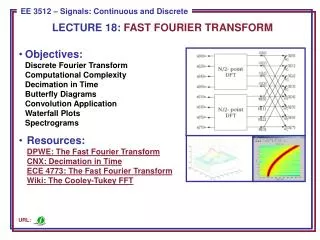
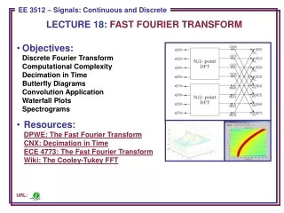
N/2 DFT x[0,2,4,6] X[0…7] • Cross feed of G[k] and H[k] in flow diagram is called a “butterfly”, due to the shape N/2 DFT x[1,3,5,7] or simplify: -1
对N=8, bit reversal (0, 1, 2, 3, 4, 5, 6, 7 is reordered to 0, 4, 2, 6, 1, 5, 3, 7)
因为WN/2 = -1, Xk0和Xk1具有周期N/2, Diagrammatically (butterfly), There are N/2 butterflies for this stage of the FFT, and each butterfly requires one multiplication The splitting of {Xk} into two half-size DFTs can be repeated on Xk0 and Xk1 themselves,
The FFT for eight data values d1,d2,…,d7 proceeds as follows. 参考 P55, C.W.Ueberhuber,Numerical Computation 2,Springer 1995.
{Xk00} is the N/4-point DFT of {x0, x4,…, xN-4}, • {Xk01} is the N/4-point DFT of {x2, x6,…, xN-2}, • {Xk10} is the N/4-point DFT of {x1, x5,…, xN-3}, • {Xk11} is the N/4-point DFT of {x3, x7,…, xN-1}.
定义 c=[0 2 4 6 1 3 5 7] 这里四页内容选自G.H.Golub,C.F.Van Loan的《矩阵计算》。
设 n=2t function y=fft(x,n) if n=1 y=x else m=n/2; w=e-i2πn yT=fft(x(0:2:n),m) yB=fft(x(1:2:n),m) d=[1,w,…,wm-1]T z=d.*yB y=[yT+z; yB+z] end 它有一种非循环的实现方式,可用 的分解来描述: 其中 称为反位置换(bit reversal permutation).
fftgui(y)产生4个plots: real(y), imag(y), real(fft(y)), imag(fft(y)) print -deps FftGui.eps print –depsc2 FftGui.eps 以下部分内容选自Moler的书《Numerical Computing with Matlab》。
Some symmetries in the FFT. Ignoring the first point in each plot, the real part is symmetric about the Nyquist point and the imaginary part is antisymmetric about the Nyquist point. More precisely, 若y是长度为n的实向量,Y=fft(y),则 real(Y0) = ∑yj imag(Y0) = 0 real(Yj) = real(Yn-j), j=1,…,n/2 imag(Yj) = -imag(Yn-j),j=1,…,n/2
% the sampling rate. Fs = 32768; t = 0:1/Fs:0.25; % the button in position (k,j) for k=1:4 for j=1:3 y1 = sin(2*pi*fr(k)*t); y2 = sin(2*pi*fc(j)*t); y = (y1 + y2)/2; input('Press any key:)'); sound(y,Fs) end end 697 770 852 941 1209 1336 1477
Forcenturies,peoplehavenotedthatthefaceofthesunisnotconstantoruniforminappearance,butthatdarkerregionsappearatrandomlocationsonacyclicalbasis. In1848,Rudolf Wolfer proposed a rule that combined the number and size of these sunspots into a single index. load sunspot.dat t = sunspot(:,1)'; wolfer = sunspot(:,2)'; n = length(wolfer); c = polyfit(t,wolfer,1); trend = polyval(c,t); plot(t,[wolfer; trend],'-', t,wolfer,'k.')
Nowsubtract off thelineartrendandtaketheFFT. y = wolfer - trend; Y = fft(y); Fs = 1; % Sample rate f = (0:n/2)*Fs/n; pow = abs(Y(1:n/2+1)); plot([f; f],[0*pow; pow],'c-', … f,pow,'b.', ... 'linewidth',2, 'markersize',16)
plot(fft(eye(17))) axis square
Chebyshev Polynomial 递推关系: 满足微分方程: 扩充到复平面 扩充到|z|>1 第二类Chebyshev多项式
shg,hold on fplot('x',[-1,1]) fplot('2*x^2-1',[-1,1]) fplot('4*x^3-3*x',[-1,1]) fplot('8*x^4-8*x^2+1',[-1,1]) fplot('16*x^5-20*x^3+5*x',[-1,1])
“We do not make things, We make things better.”