The Fast Fourier Transform
The Fast Fourier Transform. Outline and Reading. Polynomial Multiplication Problem Primitive Roots of Unity (§10.4.1) The Discrete Fourier Transform (§10.4.2) The FFT Algorithm (§10.4.3) Integer Multiplication (§10.4.4) Java FFT Integer Multiplication (§10.5). Polynomials. Polynomial:

The Fast Fourier Transform
E N D
Presentation Transcript
Outline and Reading • Polynomial Multiplication Problem • Primitive Roots of Unity (§10.4.1) • The Discrete Fourier Transform (§10.4.2) • The FFT Algorithm (§10.4.3) • Integer Multiplication (§10.4.4) • Java FFT Integer Multiplication (§10.5) FFT
Polynomials • Polynomial: • In general, FFT
Polynomial Evaluation • Horner’s Rule: • Given coefficients (a0,a1,a2,…,an-1), defining polynomial • Given x, we can evaluate p(x) in O(n) time using the equation • Eval(A,x): [Where A=(a0,a1,a2,…,an-1)] • If n=1, then return a0 • Else, • Let A’=(a1,a2,…,an-1) [assume this can be done in constant time] • return a0+x*Eval(A’,x) FFT
Polynomial Multiplication Problem • Given coefficients (a0,a1,a2,…,an-1) and (b0,b1,b2,…,bn-1) defining two polynomials, p() and q(), and number x, compute p(x)q(x). • Horner’s rule doesn’t help, since where • A straightforward evaluation would take O(n2) time. The “magical” FFT will do it in O(n log n) time. FFT
Polynomial Interpolation & Polynomial Multiplication • Given a set of n points in the plane with distinct x-coordinates, there is exactly one (n-1)-degree polynomial going through all these points. • Alternate approach to computing p(x)q(x): • Calculate p() on 2n x-values, x0,x1,…,x2n-1. • Calculate q() on the same 2n x values. • Find the (2n-1)-degree polynomial that goes through the points {(x0,p(x0)q(x0)), (x1,p(x1)q(x1)), …, (x2n-1,p(x2n-1)q(x2n-1))}. • Unfortunately, a straightforward evaluation would still take O(n2) time, as we would need to apply an O(n)-time Horner’s Rule evaluation to 2n different points. • The “magical” FFT will do it in O(n log n) time, by picking 2n points that are easy to evaluate… FFT
Primitive Roots of Unity • A number w is a primitive n-th root of unity, for n>1, if • wn = 1 • The numbers 1, w, w2, …, wn-1 are all distinct • Example 1: • Z*11: • 2, 6, 7, 8 are 10-th roots of unity in Z*11 • 22=4, 62=3, 72=5, 82=9 are 5-th roots of unity in Z*11 • 2-1=6, 3-1=4, 4-1=3, 5-1=9, 6-1=2, 7-1=8, 8-1=7, 9-1=5 • Example 2: The complex number e2pi/n is a primitive n-th root of unity, where FFT
Properties of Primitive Roots of Unity • Inverse Property: If w is a primitive root of unity, then w -1=wn-1 • Proof: wwn-1=wn=1 • Cancellation Property: For non-zero -n<k<n, • Proof: • Reduction Property: If w is a primitve (2n)-th root of unity, then w2 is a primitive n-th root of unity. • Proof: If 1,w,w2,…,w2n-1 are all distinct, so are 1,w2,(w2)2,…,(w2)n-1 • Reflective Property: If n is even, then wn/2 = -1. • Proof: By the cancellation property, for k=n/2: • Corollary: wk+n/2= -wk. FFT
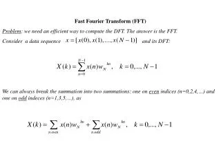
The Discrete Fourier Transform • Given coefficients (a0,a1,a2,…,an-1) for an (n-1)-degree polynomial p(x) • The Discrete Fourier Transform is to evaluate p at the values • 1,w,w2,…,wn-1 • We produce (y0,y1,y2,…,yn-1), where yj=p(wj) • That is, • Matrix form: y=Fa, where F[i,j]=wij. • The Inverse Discrete Fourier Transform recovers the coefficients of an (n-1)-degree polynomial given its values at 1,w,w2,…,wn-1 • Matrix form: a=F -1y, where F -1[i,j]=w-ij/n. FFT
Correctness of the inverse DFT • The DFT and inverse DFT really are inverse operations • Proof: Let A=F -1F. We want to show that A=I, where • If i=j, then • If i and j are different, then FFT
Convolution • The DFT and the inverse DFT can be used to multiply two polynomials • So we can get the coefficients of the product polynomial quickly if we can compute the DFT (and its inverse) quickly… FFT
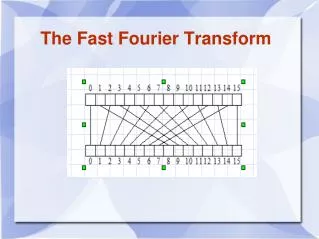
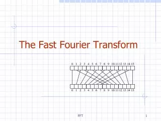
The Fast Fourier Transform • The FFT is an efficient algorithm for computing the DFT • The FFT is based on the divide-and-conquer paradigm: • If n is even, we can divide a polynomial into two polynomials and we can write FFT
The FFT Algorithm The running time is O(n log n). [inverse FFT is similar] FFT
Multiplying Big Integers • Given N-bit integers I and J, compute IJ. • Assume: we can multiply words of O(log N) bits in constant time. • Setup: Find a prime p=cn+1 that can be represented in one word, and set m=(log p)/3, so that we can view I and J as n-length vectors of m-bit words. • Finding a primitive root of unity. • Find a generator x of Z*p. • Then w=xc is a primitive n-th root of unity in Z*p (arithmetic is mod p) • Apply convolution and FFT algorithm to compute the convolution C of the vector representations of I and J. • Then compute • K is a vector representing IJ, and takes O(n log n) time to compute. FFT
Java Example: Multiplying Big Integers • Setup: Define BigInt class, and include essential parameters, including the prime, P, and primitive root of unity, OMEGA. 10; FFT
Java Integer Multiply Method • Use convolution to multiply two big integers, this and val: FFT
Java FFT in Z*p FFT
Non-recursive FFT • There is also a non-recursive version of the FFT • Performs the FFT in place • Precomputes all roots of unity • Performs a cumulative collection of shuffles on A and on B prior to the FFT, which amounts to assigning the value at index i to the index bit-reverse(i). • The code is a bit more complex, but the running time is faster by a constant, due to improved overhead FFT
Experimental Results • Log-log scale shows traditional multiply runs in O(n2) time, while FFT versions are almost linear FFT