Fast Fourier Transform: Efficiency and Applications
140 likes | 396 Vues
Learn about the Fast Fourier Transform (FFT) and its computational efficiency in reducing complex multiplications, along with its applications in convolution, waterfall plots, and spectrograms.

Fast Fourier Transform: Efficiency and Applications
E N D
Presentation Transcript
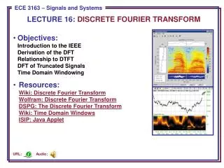
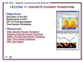
LECTURE 18: FAST FOURIER TRANSFORM • Objectives:Discrete Fourier TransformComputational ComplexityDecimation in TimeButterfly DiagramsConvolution ApplicationWaterfall PlotsSpectrograms • Resources:DPWE: The Fast Fourier TransformCNX: Decimation in TimeECE 4773: The Fast Fourier TransformWiki: The Cooley-Tukey FFT URL:
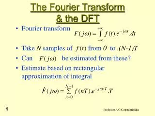
The Discrete Fourier Transform • Recall our definition for the Discrete Fourier Transform (DFT): • The computation for Xk requires N2 complex multiplications that require four multiplications of real numbers per complex multiplication. • The Fast Fourier Transform (FFT) is an approach to reduce the computational complexity that produces the same result as a DFT (same result, significantly fewer multiplications). • To simplify notation, define: • We can rewrite the DFT equations:
Decimation in Time (Radix 2) • Let’s explore an approach that subdivides time interval into successively smaller intervals. Assume N, the size of the DFT, is an even integer so that N/2 is also an integer. Define two auxiliary signals: • Let Ak and Bk denote two (N/2)-point DFTs of a[n] and b[n]: • We can show that these are related to the DFT by the following equations: • The computation of Ak and Bk each requires (N/2)2 = N2/4 multiplications. The scaling by requires N/2 additional multiplications. The total computation is N2/2+N/2 multiplications, which represents N2/2-N/2 fewer multiplications than the N2 multiplications required by the DFT. • For N= 128, this is a savings of 8,128 multiplications (16,384vs. 8,256).
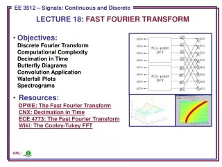
Block Diagram of an FFT Algorithm • If N is a power of 2 (e.g., N= 2q), we can repeat this process to further reduce the computations. The overall complexity reduces from N2 to (Nlog2N)/2.
Bit Reversing • Note that the inputs have been shuffled so that the outputs are produced in the correct order. • This can be represented as a bit-reversing process:
Application – Convolution • Given two time-limited signals: • let r equal the smallest possible integer such that N + Q < 2r. Let L = 2r. • We can pad these signals with zeros to make them the same length so that we can apply an FFT: • The convolution of these two (zero-padded) signals computed using a convolution sum requires L2 /2 + 3L/2 multiplications. Computing the convolution using the FFT requires (3L/2)log2L + L multiplications. • Example: Consider the convolution of a pulse and a truncated exponential. • What is the effect of truncating the exponential in the frequency domain?
Application – Convolution (Cont.) • We can select an FFT Order as follows: • N = 16 • Q = 16 (an approximation) • N + Q = 32 =2**5 L = 5 • The MATLAB code to generate theL-point DFT using the function fft() is: • N = 0:16; L = 32; • v = (0.8).^n; • Vk = fft(v, L); • x = [ones(1, 10)] • Xk = fft(x, L); • The output can be generated bymultiplying the frequency responses,and taking the inverse FFT: • Yk = Vk.*Xk;y = ifft(Yk, L); • This can be validated by using the time-domainconvolution function from Chapter 2.
Application – Waterfall Plots • Often we will used an overlapping frame-based analysis to compute the spectrum as a function of time. • This approach is used in many disciplines (e.g., graphic equalizer in audio systems). • One popular visualization is referred to as a waterfall plot.
Applications of the FFT – The Spectrogram • Another very important visualization tool is the spectrogram, a time-frequency plot of the spectrum in which the spectral magnitude is plotted as a grayscale value or color.
Applications to Speech Processing • The choice of the length of the FFT can produce dramatically different views of your signal. • For speech signals, a 6 ms window (48 samples at 8 kHz) allows visualization of individual speech sounds (phonemes). • A longer FFT length (240 samples – 30 ms at 8 kHz) allows visualization of the fundamental frequency and its harmonics, which is related to the vibration of the vocal chords. • Such time-frequency displays need not be limited to the Fourier transform. For example, wavelets are a popular alternative.
Spectrograms in MATLAB • MATLAB contains a wide variety of visualization tools including a spectrogram function. • MATLAB can read several file formats directly, including .wav files. • Several aspects of the spectrogram can be programmed, including the color map and the analysis window.
Summary • Introduced a decimation-in-time approach to fast computation of the DFT known as the Fast Fourier Transform. • Discussed the computational efficiency. • Demonstrated application of this to convolution. • Introduced applications of the convolution known as the waterfall plot and the spectrogram.