Download
1 / 31
610 likes | 1.73k Vues
Chapter 8 Fast Fourier Transform (FFT) Section 9.1-9.4, 10.1. 8.1 Introduction 8.2 Goertzel Algorithm 8.3 Fast Fourier Transform (FFT) 8.4 Inverse FFT (IFFT) 8.5 Signal Analysis using DFT. 8.1.1 DFT Expression. Consider how complicated this is when x [ n ] is complex.

E N D
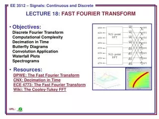
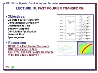
Chapter 8 Fast Fourier Transform (FFT)Section 9.1-9.4, 10.1 • 8.1 Introduction • 8.2 Goertzel Algorithm • 8.3 Fast Fourier Transform (FFT) • 8.4 Inverse FFT (IFFT) • 8.5 Signal Analysis using DFT
8.1.1 DFT Expression Consider how complicated this is when x[n] is complex. Represent x[n]=Re{x[n]}+j Im{x[n]}. We have the expression:
8.1.2 DFT Computational Complexity • For each K we have 4N real multiplications, 4N-2 real adds. • For all N of X[k] we have • N(4N) = 4N2 real multiplication • N(4N-2) = 4N2 -2N real adds • Example. N=1000 • # multiplications = 4,000,000 ! • # additions 4,000,000 • The computational complexity is O(N2). As N increase, the order becomes huge! • Storage Requirements (memory): x[n] -N values (complex), WN-N values (complex), which can be reduced due to periodicity and symmetry.
8.1.3 DFT Symmetry and Periodicity Properties Symmetry and Periodicity Periodic in both k and n with period N Example N=8
8.1.4 Symmetry and Periodicity Properties Based on the symmetry, we can write for real part: Re{x[n]}Re{WNkn}+ Re{x[N-n]}Re{WNk(N-n) } Group terms, drop one multiplication we get: (Re{x[n]}+ Re{x[N-n]})Re{WNkn} Since Re{WNkn}= Re{WNk(N-n)} Similarly for other three terms, and this results in a reduction by 50% of real multiplications without really doing anything. However, the overall complexity is still O(N2) The periodicity property is better that leads to the Fast Fourier Transform (FFT) with O(Nlog(N))
8.1.5 FFT History Known for many years Gauss 1805 Runge 1905 Danielson and Lanczos (1942) Hand calculation of the DFT Relatively short sequence Cooly & Tukey – 1965 Modern algorithm that could decompose a DFT into a sum of shorter DTFs When N is a composite number, i.e., the product of two or more integers.
8.1.6 FFT Principles Decompose a sequence into successively smaller sequence to reduce overall computation . Example: Consider N=100 Brute Force O(N2)=10000 If we can break this into 2 (50 point) DFTs, then: O(502) + O(502) =5000<10000 ! Decompose further, gaining each time. Two basic classes Decimation in time (DIT) Decimation in frequency (DIF)
8.2.1 Goertel Algorithm: Periodicity The Goertel algorithm is an example of how the periodicity of the sequence can be used to reduce computation. To suggest the final result, let us define the sequence It can be interpreted as a discrete convolution of the finite duration sequence with the sequence Consequentially, can be viewed as the response of a system with impulse response to a finite-length input x[n]. In particular, X[k] is the value of the output when n=N.
Z-1 8.2.2 Goertel Algorithm: Complexity For a particular value of k, we need 4N real multiplications and 4N real additions to compute X[k]. This procedure is slightly less efficient than the direct method. It avoids the computation or storage of the coefficient , since these quantities are implicitly computed by the recursion.
8.2.3 Goertel Algorithm: Complexity Reduction 2(N+2) real multiplications 4(N+1) real additions
8.2.4 Goertel Algorithm: Comments • In either the direct method or the Goertzel method, we do not need to evaluate X[k] at all N values. • We can evaluate X[k] for any M values of k, with each DFT value being computed by a recursive system. • This is slightly less efficient than DFT performed directly. • But, WNkn does not need to be computed and stored in advance due to recursive nature of the algorithm. • Advantage: Goertzel’s algorithm can be used to compute efficiently a small number of DFT coefficients. • Next – the real FFT
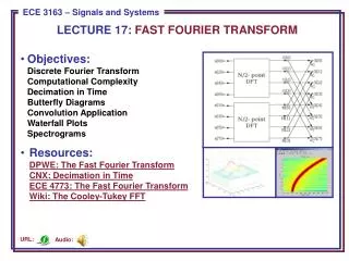
8.3.1 DIT-FFT: Concepts • Decimation in Time (DIT) FFT – Classical approach: • Based on decomposing x[n] into small sequences • Exploits both periodicity and symmetry of W • Usually consider N=2v so that we can successively subdivide by factor of 2 (v times) all the way down to length – 2 subsequences. • Divide into even and odd indexed points • Let N=2v
8.3.2 DIT-FFT: Formulas So we can write Want to write this as a sum of N/2 points DFT
8.3.2 DIT-FFT: Formulas (Cont’d) • Rewrite • Where G[k] and H[k] are N/2 point DFT • G[k] and H[k] are both periodic with period N/2 • So, must be computed over only N/2 points (not N) • X(k) is still N points long. • Lets check the flow diagram
8.3.3 DIT-FFT: Flow Graph Because of periodicity G[4]=G[0] H[4]=H[0] G[5]=G[1] H[5]=H[1] G[6]=G[2] H[6]=H[2] ….
8.3.4 DIT-FFT: Reduced Complexity • Consider computation: • Recall that DFT is O(N2) • Now length is N/2, not N, but there are two N/2 point DFTs • At first (Complex) • N2 multiplications and adds (each) • Now, 2*(N/2)2 = N2/2 multiplications and additions (each) • Plus N complex multiplications for W • Plus N complex additions • Total = N+N2/2 complex multiplications and adds. • Since N+N2/2 < N2 ! A savings for N=2v. • We can continue this decomposition process and get more savings, if N/2 is even and greater than 2.
8.3.5 DIT-FFT: Procedure • Assume N=8 • Stage I : Form two 4 point DFTs, plus combining algebra • Stage II: Split 4-point DFTs into four 2-point DFTs, plus combining algebra • Would continue if N>8 • Consider the two 4-point DFTs
8.3.5 DIT-FFT: Procedure (Cont’d) • Where • This represents the 4-point DFTs as four 2-point DFTs plus 2 stages of combining algebra • If N=2v, it will take v stages to do this completely. • log2N decomposition to get down to 2-point DFTs, now require 4(N/4)2+2(N/2)+N=N2/4+N+N<N2 • A 2-point DFT – what is the simplest stage like? p[0] p[1] P[0]=p[0]+p[1] P[1]=p[0]+W21p[1]
xm[p] xm[q] Xm+1[p] Xm+1[q] 8.3.6 DIT-FFT: Complexity • With this decomposition, each stage requires N complex mults and ~N complex adds • There are log2N stages • Thus Nlog2N complex mults and adds, not N2 • Further reduction results in each stage of Butterflies of form as In general Xm+1 [p]=Xm [p]+WrNXm [q] Xm+1 [q]=Xm [p]+WN(r+N/2)Xm [q]
xm[p] xm[q] Xm+1[p] Xm+1[q] -1 8.3.6 DIT-FFT: Complexity (Cont’d) But Then the general Butterfly can be written as So
8.3.6 DIT-FFT: Complexity (Cont’d) • This signal flow graph saves one complex multiply per butterfly – which cuts the total by half • # complex mults = N/2 log2N • # complex adds = Nlog2N • As opposed to N2 of the DFT direct computation. • Consider reductions:
8.3.7 DIT-FFT: In-Place Computations • Due to “flow of calculation” from left to right, 2-point calculations in each Butterfly – only a single complex storage array is needed in the computation • Bit reward ordering: data is stored in “bit-reversed” order due to the even/odd splits on the data.
8.3.8 Decimation-In-Frequency (DIF) • Subdivide X[k] into successively smaller subsequences • Let N=2v • These are 2 N/2 point DFTs
8.4.1 Inverse FFT: Ideas • Want to compute IDFT using FFT • Multiply IDFT by N 2. Take the complex conjugate 3. Take the conjugate again which is the DFT of X*[k] 4. Divided by N
8.4.2 Inverse FFT: Procedure and Example • Get X*[k]; • Compute FFT(X*[k]); • Compute conjugate to get Nx[n]; • Divide result by N. Original Image A FFT(A) Sine Wave B FFT(B) A+B FFT(A+B) FFT(A+B)-FFT(B) IFFT[FFT(A+B)-FFT(B)]
8.5.1 Signal Analysis using DFT • Anti-aliasing filter is to incorporated to eliminate or minimize the effect of aliasing when the continuous-time is converted to a sequence. • The need for multiplication of x[n] by w[n] is a consequence of the finite-length requirement. • A finite-duration window w[n] is applied to x[n] prior to computation of the DFT in order to smooth sharp peaks and discontinuities in . • The C/D conversion is represented in the frequency-domain as
Illustration of the Fourier transforms: • Fourier transform of continuous-time input signal. • Frequency response of anti-aliasing filter. • Fourier transform of output of anti-aliasing filter. • Fourier transform of sampled signal. • Fourier transform of window sequence. • Fourier transform of windowed segment and frequency samples obtained using DFT samples.