Fast Fourier Transform (FFT) Algorithms
Fast Fourier Transform (FFT) Algorithms. Relation to the z-transform. The DFS X(k) represents N evenly spaced samples of the z-transform X(z) around the unit circle. Relation to the DTFT. The DFS is obtained by evenly sampling the DTFT at w 1 intervals.

Fast Fourier Transform (FFT) Algorithms
E N D
Presentation Transcript
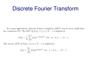
Relation to the z-transform The DFS X(k) represents N evenly spaced samples of the z-transform X(z) around the unit circle.
Relation to the DTFT The DFS is obtained by evenly sampling the DTFT at w1 intervals. The interval w1 is the sampling interval in the frequency domain. It is called frequency resolution because it tells us how close are the frequency samples.
Sampling and construction in the z-domain DFS & z-transform IDFS
Comments • When we sample X(z) on the unit circle, we obtain a periodic sequence in the time domain. • This sequence is a linear combination of the original x(n) and its infinite replicas, each shifted by multiples of N or –N. • If x(n)=0 for n<0 and n>=N, then there will be no overlap or aliasing in the time domain.
Comments RN(n) is called a rectangular window of length N. THEOREM1: Frequency Sampling If x(n) is time-limited (finite duration) to [0,N-1], then N samples of X(z) on the unit circle determine X(z) for all z.
Reconstruction Formula Let x(n) be time-limited to [0,N-1]. Then from Theorem 1 we should be able to recover the z-transform X(z) using its samples X~(k). WN-kN=1
Examples 5.6 5.7 Comments • Zero-padding is an operation in which more zeros are appended to the original sequence. The resulting longer DFT provides closely spaced samples of the discrete-times Fourier transform of the original sequence. • The zero-padding gives us a high-density spectrum and provides a better displayed version for plotting. But it does not give us a high-resolution spectrum because no new information is added to the signal; only additional zeros are added in the data. • To get high-resolution spectrum, one has to obtain more data from the experiment or observations.
Traditional cache solution: Blocking Size 8 DFT p = 2 (radix 2) Size 4 DFT Size 4 DFT Size 2 DFT Size 2 DFT Size 2 DFT Size 2 DFT breadth-first, but with blocks of size = cache …requires program specialized for cache size
eventually small enough to fit in cache …no matter what size the cache is Recursive Divide & Conquer is Good [Singleton, 1967] (depth-first traversal) Size 8 DFT p = 2 (radix 2) Size 4 DFT Size 4 DFT Size 2 DFT Size 2 DFT Size 2 DFT Size 2 DFT
Goal of an Efficient computation • The total number of computations should be linear rather than quadratic with respect to N. • Most of the computations can be eliminated using the symmetry and periodicity properties CN=N×log2N If N=2^10, CN=will reduce to 1/100 times. Decimation-in-time: DIT-FFT, decimation-in-frequency: DIF-FFT
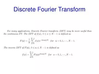
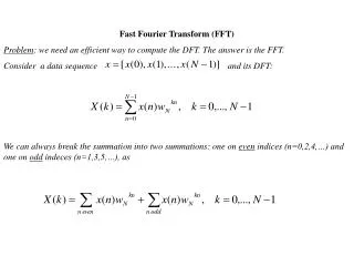
Efficient Computation of Discrete Fourier Transform • Electrical sciences is full of signal processing • Digital computers paved way for reliable signal processing • DFT plays an important role and needs efficient procedure for computation of X(k),
Direct Computation of the DFT • To indicate the importance of efficient computation schemes, it is instructive to consider the direct evaluation of the DFT equation, Eq.(2.1). Since x(n) may be complex, we can write
From Eq.(2.2) it is clear that for each value of k, the direct computation of X(k) requires 4N real multiplications and (4N-2) real additions. • Total 4N2 real multiplications and N(4N-2) real additions. • The amount of time required for computation becomes large.
Most approaches of improving the efficiency of the computation of the DFT exploit one or both of the following special properties of the quantity
Cooley and Tukey published an algorithm for computation of DFT that is applicable when N is a composite number. • Number of such computational algorithms are known as fast Fourier transform, or simply FFT algorithms.
Radix-2 FFT Algorithms • Let N=2v; then we choose M=2 and L=N/2 and divide x(n) into two N/2-point sequence. • This procedure can be repeated again and again. At each stage the sequences are decimated and the smaller DFTs combined. This decimation ands after v stages when we have N one-point sequences, which are also one-point DFTs. • The resulting procedure is called the decimation-in-time FFT (DIF-FFT) algorithm, for which the total number of complex multiplications is: CN=Nv= N*log2N; • using additional symmetries: CN=Nv= N/2*log2N • Signal flowgraph in Figure 5.19
Decimation-in-frequency FFT • In an alternate approach we choose L=2, M=N/2 and follow the steps in (5.49). • We can get the decimation-frequency FFT (DIF-FFT) algorithm. • Its signal flowgraph is a transposed structure of the DIT-FFT structure. • Its computational complexity is also equal to CN=Nv= N/2*log2N
Radix-2 FFT Algorithms • To achieve the dramatic increase in efficiency, it is necessary to decompose the DFT computation into successively smaller DFT computations. In this process we exploit both the symmetry and the periodicity of the complex exponential .
Decimation-in-time FFT Algorithm • The principle of decimation-in-time is most conveniently illustrated by considering the special case of N an integer power of 2; i.e. • Since N is an even integer, we can consider computing X(k) by separating x(n) into two N/2-point sequences consisting of the even-numbered points in x(n) and the odd-numbered points in x(n). With X(k) given by
Separating x(n) into even-numbered and odd-numbered points, we obtain or with the substitution of variables n=2r for an even and n=2r+1 for odd ,
But Consequently, Eq. (2.4) can be written as Each of the sums in Eq.(2.5) is recognized as an N/2-point DFT. Each of sums need only be computed for k between 0 and N/2. Since G(k) and H(k) are each periodic in k with period N/2.
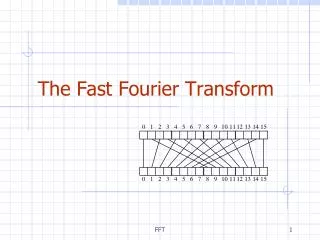
The computational flow or the signal flow in computing X(k) according to Eq. (2.5) for an 8-point sequence, i.e. N=8 is shown in Figure below. .
Equation (2.5) corresponds to breaking the original N-point DFT computation into two N/2-point DFT computations. Each of the N/2-point DFT computations can be further broken into two N/4-point DFTs. Thus G(k) and H(k) in Eq.(2.5) would be computed as indicated next.
Similarly, where g(r)=x(2r) and h(r)=h(2r+1).
If the 4-point DFTs in Figure (2.1) are computed according to Eqs. (2.6) and (2.7), then that computation would be carried out as indicated in Figure (2.2).
Inserting the computation indicated in Figure (2.2) into the flow graph of Figure (2.1), we obtain the complete flow graph of Figure (2.3). We have used the fact that N/2 = WN2.
In-place Computations • In view of Figure (2.4), the Figure (2.3) gives the complete computational flow graph for the N-point computation of DFT of N-point sequence, for N=8. • An interesting by-product of this derivation is that, this flow graph, in addition to describing efficient procedure for computing the DFT, also suggests a useful way of storing the original data and storing the results of the computation in the intermediate arrays.
For N=8, N/4-point DFT becomes 2-point DFT. The 2-point DFT of, for example, x(0) and x(4) is depicted in Figure (2.4).
We shall denote the sequence of complex numbers resulting from the mth stage of computation as Xm(l), where l=0,1,..,N-1, and m=1,2,.., forming an input to the (m+1)st stage and producing an output Xm+1(l) as the output from the (m+1)st stage of computations, it can be seen that the basic computation in flow graph of Figure (2.3)
The equations represented by this flow graph are Because of the appearance of the flow graph of Figure (2.5), this computation is referred as a butterfly computation. Equations (2.8) suggest a means of reducing the number of complex multiplications by a factor of 2. To see this we note that
So the equations (2.8) become Equations (2.9) are represented in the flow graph of Figure (2.6).
Combining the observations in Figures (2.6), (2.5), (2.4) and (2.3), the efficient FFT algorithm in the computational flow graph representation for N=8 is obtained as shown in Figure (2.7).The algorithm requires N/2log2N complex multiplications and N log2 N complex additions.
Decimation-in-Frequency FFT Algorithm • The decimation-in-time FFT algorithms were all based upon the decomposition of the DFT computation by forming smaller and smaller subsequences. • Alternatively decimation-in-frequency FFT algorithms are all based upon decomposition of the DFT computation over X(k). For N, a power of 2 i.e. we divide the input sequence into first half and the last half of points so that
Separating k-even and k-odd, i.e. k=2r and k=2r+1, representing the even-numbered points and the odd-numbered points, respectively, so that
Thus on the basis of Equations (2.11) and (2.12) with and The DFT can be computed by first forming the sequences g(n) and h(n), then computing h(n)WNn, and finally computing the N/2-point DFTs of these two sequences to obtain the even-numbered output points and odd-numbered output points, respectively.
The procedure suggested by Eqs. (2.11) and (2.12) is illustrated through signal flow graph for the case of 8-point DFT in Figure (2.8).
Proceeding in a manner similar to that followed in deriving the decimation-in-time algorithm, the final signal flow graph for computation is shown in Figure (2.9).
By counting the arithmetic operations in Figure (2.9), and generalizing, we see that the computation of Figure (2.9) requires N/2log2N complex multiplications and Nlog2N complex additions. Thus the total computation is the same for decimation-in-frequency and decimation-in-time algorithms. • Similar to decimation-in-time algorithm the computational flow graph shown in Figure (2.9) will indicate the in-place computation capability of decimation-in-frequency algorithm. • Figure (2.9) is the transpose of Figure (2.7).
Decimation-In-Time FFT Algorithms • Makes use of both symmetry and periodicity • Consider special case of N an integer power of 2 • Separate x[n] into two sequence of length N/2 • Even indexed samples in the first sequence • Odd indexed samples in the other sequence • Substitute variables n=2r for n even and n=2r+1 for odd • G[k] and H[k] are the N/2-point DFT’s of each subsequence
8-point DFT example using decimation-in-time Two N/2-point DFTs 2(N/2)2 complex multiplications 2(N/2)2 complex additions Combining the DFT outputs N complex multiplications N complex additions Total complexity N2/2+N complex multiplications N2/2+N complex additions More efficient than direct DFT Repeat same process Divide N/2-point DFTs into Two N/4-point DFTs Combine outputs Decimation In Time
Decimation In Time Cont’d • After two steps of decimation in time • Repeat until we’re left with two-point DFT’s
Decimation-In-Time FFT Algorithm • Final flow graph for 8-point decimation in time • Complexity: • Nlog2N complex multiplications and additions
Butterfly Computation • Flow graph constitutes of butterflies • We can implement each butterfly with one multiplication • Final complexity for decimation-in-time FFT • (N/2)log2N complex multiplications and additions
In-Place Computation • Decimation-in-time flow graphs require two sets of registers • Input and output for each stage • Note the arrangement of the input indices • Bit reversed indexing
Decimation-In-Frequency FFT Algorithm • The DFT equation • Split the DFT equation into even and odd frequency indexes • Substitute variables to get • Similarly for odd-numbered frequencies
Decimation-In-Frequency FFT Algorithm • Final flow graph for 8-point decimation in frequency
FFT vs. DFT • The FFT is simply an algorithm for efficiently calculating the DFT • Computational efficiency of an N-Point FFT: • DFT: N2 Complex Multiplications • FFT: (N/2) log2(N) Complex Multiplications
Bit Reversal • The bit reversal algorithm used to perform the re-ordering of signals. • The decimal index, n, is converted to its binary equivalent. • The binary bits are then placed in reverse order, and converted back to a decimal number. • Bit reversing is often performed in DSP hardware in the data address generator (DAG).
DIT FFT • Input signal must be properly re-ordered using a bit reversal algorithm • In-place computation • Number of stages: log2 N • Stage 1: all the twiddle factors are 1 • Last Stage: the twiddle factors are in sequential order