Probability and Statistics for Engineers
350 likes | 848 Vues
Probability and Statistics for Engineers. Descriptive Statistics Measures of Central Tendency Measures of Variability Probability Distributions Discrete Continuous Statistical Inference Design of Experiments Regression. Descriptive Statistics.

Probability and Statistics for Engineers
E N D
Presentation Transcript
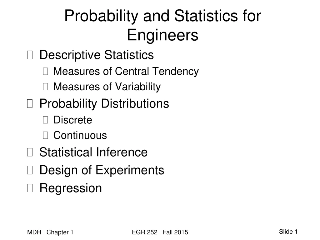
Probability and Statistics for Engineers • Descriptive Statistics • Measures of Central Tendency • Measures of Variability • Probability Distributions • Discrete • Continuous • Statistical Inference • Design of Experiments • Regression EGR 252 Fall 2015
Descriptive Statistics • Numerical values that help to characterize the nature of data for the experimenter. • Example: The absolute error in the readings from a radar navigation system was measured with the following results: • the sample mean, x = ? 17 22 39 31 28 52 147 EGR 252 Fall 2015
Calculation of Mean • Example: The absolute error in the readings from a radar navigation system was measured with the following results: _ • the sample mean, X = (17+ 22+ 39 + 31+ 28 + 52 + 147) / 7 = 48 17 22 39 31 28 52 147 EGR 252 Fall 2015
Calculation of Median • Example: The absolute error in the readings from a radar navigation system was measured with the following results: • the sample median, x = ? • Arrange in increasing order: 17 22 28 31 39 52 147 • n odd median = x (n+1)/2 , → 31 • n even median = (xn/2 + xn/2+1)/2 • If n=8, median is the average of the 4th and 5th data values. 17 22 39 31 28 52 147 ~ EGR 252 Fall 2015
Descriptive Statistics: Variability • A measure of variability • Example: The absolute error in the readings from a radar navigation system was measured with the following results: • sample range = Max – Min = 147 – 17 = 130 17 22 39 31 28 52 147 EGR 252 Fall 2015
Calculations: Variability of the Data • sample variance, • sample standard deviation, EGR 252 Fall 2015
Other Descriptors • Discrete vs Continuous • discrete: countable • continuous: measurable • Distribution of the data • “What does it look like?” EGR 252 Fall 2015
Graphical Methods – Stem and Leaf Stem and leaf plot for radar data Stem Leaf Frequency 1 7 1 2 2 8 2 3 1 9 2 4 5 2 1 6 7 8 9 10 11 12 13 14 7 1 EGR 252 Fall 2015
Graphical Methods - Histogram • Frequency Distribution (histogram) • Develop equal-size class intervals – “bins” • ‘Rules of thumb’ for number of intervals • Less than 50 observations 5 – 7 intervals • Square root of n • Interval width = range / # of intervals • Build table • Identify interval or bin starting at low point • Determine frequency of occurrence in each bin • Calculate relative frequency • Build graph • Plot frequency vs interval midpoint EGR 252 Fall 2015
Data for Histogram • Example: stride lengths (in inches) of 25 male students were determined, with the following results: • What can we learn about the distribution (shape) of stride lengths for this sample? EGR 252 Fall 2015
Constructing a Histogram • Determining frequencies and relative frequencies = 2/25 S = 25 S = 1.0 EGR 252 Fall 2015
Computer-Generated Histograms Bin Size determined using Sturges’ formula = 1+3.3 log (n) = 5.61 round to 6 EGR 252 Fall 2015
Relative Frequency Graph EGR 252 Fall 2015
Graphical Methods – Dot Diagram • Dot diagram (text) • Dotplot (Minitab) EGR 252 Fall 2015
Homework and Reading Assignment • Reading • Chapter 1: Introduction to Statistics and Data Analysis pg. 1- 30 • Problems • 1.9 pg. 17 • 1.18 pg. 31 EGR 252 Fall 2015