PAC-Bayes Risk Bounds for Sample-Compressed Gibbs Classifiers
150 likes | 286 Vues
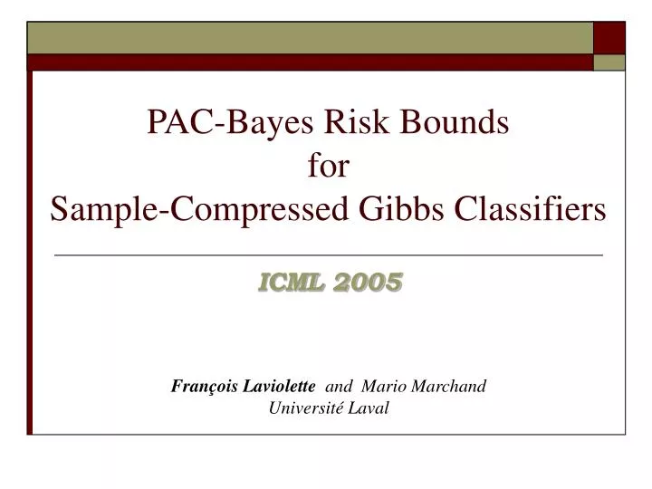
PAC-Bayes Risk Bounds for Sample-Compressed Gibbs Classifiers. ICML 2005 François Laviolette and Mario Marchand Université Laval. PLAN. The “traditional” PAC-Bayes theorem (for the usual data-independent setting )

PAC-Bayes Risk Bounds for Sample-Compressed Gibbs Classifiers
E N D
Presentation Transcript
PAC-Bayes Risk Bounds for Sample-Compressed Gibbs Classifiers ICML 2005 François Laviolette and Mario Marchand Université Laval
PLAN • The “traditional” PAC-Bayes theorem (for the usual data-independent setting ) • The “generalized” PAC-Bayes theorem (for the more general sample compression setting) • Implications and follow-ups
In particular, for Gibbs classifiers: What if we choose Pafter observing the data?
The Gibbs and the majority vote • We have a bound for GQ but we normally use instead the Bayes classifier BQ (which is the Q-weighted majority vote classifier) • Consequently R(BQ) · 2R(GQ) (can be improved with the “de-randomization” technique of Langford-Shaw-Taylor 2003) • So the PAC-Bayes theorem also gives a bound on the Majority vote classifier.
The sample compression setting • Theorem 1 is valid in the usual data-independent setting where H is defined without reference to the training data • Example: H = the set of all linear classifiers h: Rn!{-1,+1} • In the more general sample compression setting, each classifier is identified by 2 different sources of information: • The compression set: an (ordered) subset of the training set • A message string of additional information needed to identify a classifier • Theorem 1 is not valid in this more general setting
To be more precise: • In the sample compression setting, there exists a “reconstruction” function R that gives a classifier h = R(, Si) when given a compression set Si and a message string . • Recall that Si is an ordered subset of the training set S where the order is specified by i=(i1, i2, … , i|i|).
Examples • Set Covering Machines (SCM) [Marchand and Shaw-Taylor JMLR 2002] • Decision List Machines (DLM) [Marchand and Sokolova JMLR 2005] • Support Vector Machines (SVM) • Nearest neighbour classifiers (NNC) • …
Priors in the sample compression setting • The priors must be Data-independent • We will thus use priors defined over the set of all the parameters (i,) needed by the reconstruction function R, once a training set S is given.The priors should be written as:
a (the rescaled ) incorporates Occam’s principle of parsimony • The new PAC-Bayes theorem states that the risk bound for is lower than the risk bound for any .
Conclusion • The new PAC-Bayes bound • is valid in the more general sample compression setting. • incorporates automatically the Occam’s principle of parsimony • A sample compressed Gibbs classifier can have a smaller risk bound than any of its member.
The next steps • Finding derived bounds for particular sample compressed classifiers like: • majority votes of SCMs and DLMs, • SVMs • NNCs. • Developing new learning algorithms based on the theoretical information given by the bound. • A tight Risk bound for Majority vote classifiers ?
