Download
1 / 13
130 likes | 162 Vues
Bayes for Beginners. Rick Adams Methods for Dummies Wellcome Trust Centre for Neuroimaging. Reverend Thomas Bayes (1702 – 1761). ‘Essay towards solving a problem in the doctrine of chances’, published in the Philosophical Transactions of the Royal Society of London in 1764.

E N D
Bayes for Beginners Rick Adams Methods for Dummies Wellcome Trust Centre for Neuroimaging
Reverend Thomas Bayes(1702 – 1761) • ‘Essay towards solving a problem in the doctrine of chances’, published in the Philosophical Transactions of the Royal Society of London in 1764. • C18th mathematicians knew p(black) given no. of black and white balls (=Unconditional prob.) • They didn’t know p(no. black/white balls) given ball drawn is black= Conditional probability
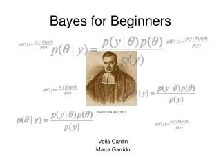
Conditional probability p(A|B) = p(A,B)/p(B) p(B|A) = p(A,B)/p(A) p(A,B) = p(A|B).p(B) = p(B|A).p(A) Therefore p(B|A) = p(A|B).p(B)/p(A) = Bayes’ theorem
Statistic terminology • P(A) is called the marginal orprior probability of A (since it is the probability of A prior to having any information about B) Similarly: • P(B): the marginal orprior probability of B • P(A|B) is called the likelihood function for A given B. • P(B|A): the posterior probabilityof B given A(since itdepends on having information about A) Bayes Rule P(B|A) = P(A|B)*P(B)/P(A) priorprobabilities of B, A (“priors”) “posterior” probability of B given A “likelihood” function for B (for fixed A)
Bayes’ Theorem for a given parameter p (data) = p (data)p () / p (data) 1/P (data) is basically a normalizing constant Posteriorlikelihood x prior The prior is the probability of the parameter and represents what was thought before seeing the data. The likelihood is the probability of the data given the parameter and represents the data now available. The posteriorrepresents what is thought given both prior information and the data just seen. It relates to the conditional density of a parameter (posterior probability) with its unconditional density (prior, since depends on information present before the experiment).
Probability as frequencies of outcomes in random experiments Probability as degrees of belief in propositions given evidence Sampling theory vs Bayes
Sampling theory vs Bayes • Sampling theory sets out to test hypothesis H1 • But in doing so it merely focuses attention on H0 (null) • It doesn’t test H1 at all!H0 is/isn’t rejected purely on the basis of how unexpected the data were to H0 ……not how much better H1 was(H0 can’t actually be accepted either: one is only ever insufficiently confident to reject it) • Furthermore, sampling theory only ever says that H0 & H1 are significantly different; but not how different
An aside on p-values • What does a p-value of 0.05 actually mean?
An aside on p-values • What does a p-value of 0.05 actually mean? • NOT p(H0 correct) [=Bayesian posterior probability]OR p(H1 incorrect) • Actually: given H0, p(data as or more extreme than those observed) were experiment repeated++ • p values are arbitrary and depend on the experimenter’s intentions • Likewise, confidence intervals… • don’t imply 95% chance the parameter is within them [=Bayesian post prob], • but actually indicate the proportion of times one would expect the true value of the parameter to fall within them were the experiment repeated++ • (i.e. the range of values which wouldn’t be rejected by a significance test)
Comparing Sampling and Bayes • A vaccine is trialled, compared with placebo. • Sampling: at sig level p=0.05 Critical value of χ2 with 1 deg freedom = 3.84Test concludes χ2 = 5.93 therefore H0 rejectedYates’ correction: χ2 = 3.33 therefore H0 accepted • Bayes:p(p(VD)<p(PD)|data) = 0.99i.e. a 99% chance that V is better than P
Model comparison • Bayesian methods allows to comparep(disease|P) and p(disease|V) • p(disease|P) / p(disease|V)= 0.6 / 0.4ie prior probability over H1 & H0 was 50:50,it is now 60:40 • Bayesian methods quantify the weakness of the evidence
Medical example • Disease present in 0.5% population (i.e. 0.005) • Blood test is 99% accurate (i.e. 0.99) • False positive 5% (i.e. 0.05) Q: If someone tests positive, what is the probability that they have the disease? • P(B|A) = P(A|B).P(B) / P(A) • P(disease|+ve) = P(+ve|disease) x P(disease) / P(+ve) = 0.99 x 0.005 / (0.99x0.005)+(0.05x0.995) = 0.00495 / 0.00495 + 0.04975 = 0.00495 / 0.0547 = 0.0905
Where is Bayesian probability useful? • In diagnostic cases: • We want to know p(Disease|Symptom) • We often know p(Symptom|Disease) from published data • Same goes for p(Disease|Test result) • In scientific cases: • We want to know p(Hypothesis|Result) • We may know p(Result|Hypothesis) – this is often statistically calculable, as when we have a p-value • Model comparison (A vs B) – there is no way to do this classically • When accepting the null is impossible (see later) • In general: it allows us to reason with unknown probabilities and quantifies uncertainty