Understanding Bayes' Theorem: Applications in Statistics and Medical Testing
This presentation introduces Bayes’ Theorem, focusing on its significance in calculating conditional probabilities. It provides clear definitions of essential terms, like P(A), P(A|B), and P(B|A), and illustrates the theorem’s application through real-world examples, particularly in medical testing for breast cancer. By analyzing probabilities before and after screenings, we demonstrate how Bayes’ Rule can inform decision-making in healthcare. Learn how prior and conditional probabilities interact to yield insights vital for diagnostics and probability assessments.


Understanding Bayes' Theorem: Applications in Statistics and Medical Testing
E N D
Presentation Transcript
Bayes for Beginners Presenters: Shuman ji & Nick Todd
Statistic Formulations. P(A): probability of event A occurring P(A|B): probability of A occurring given B occurred P(B|A): probability of B occurring given A occurred P(A,B): probability of A and B occurring simultaneously (joint probability of A and B) Joint probability of A and B P(A,B) = P(A|B)*P(B) = P(B|A)*P(A)
Bayes Rule • True Bayesians actually consider conditional probabilities as more basic than joint probabilities . It is easy to define P(A|B) without reference to the joint probability P(A,B). To see this note that we can rearrange the conditional probability formula to get: • P(A|B) P(B) = P(A,B) by symmetry: • P(B|A) P(A) = P(A,B) • It follows that: • which is the so-called Bayes Rule. • Thus, Bayes Rule is a simple mathematical formula used for calculating conditional probabilities
Bayesian Reasoning ASSUMPTIONS P(A) =1% of women aged forty who participate in a routine screening have breast cancer P(B|A)=80% of women with breast cancer will get positive tests 9.6% of women without breast cancer will also get positive tests EVIDENCE A woman in this age group had a positive test in a routine screening PROBLEM What’s the probability that she has breast cancer? = proportion of cancer patients with positive results, within the group of All patients with positive results --- P(A|B) P(B)= proportion of all patients with positive results
Bayesian Reasoning ASSUMPTIONS 100 out of 10,000 women aged forty who participate in a routine screening have breast cancer 80 of every 100 women with breast cancer will get positive tests 950 out of 9,900 women without breast cancer will also get positive tests PROBLEM If 10,000 women in this age group undergo a routine screening, about what fraction of women with positive tests will actually have breast cancer?
Bayesian Reasoning Before the screening: 100out of 10000women with breast cancer 9,900out of 10000women without breast cancer After the screening: A = 80out of 10000women with breast cancer and positive test B = 20 out of 10000 women with breast cancer and negative test C = 950out of 10000 women without breast cancer and positive test D = 8,950out of 10000women without breast cancer and negative test All patients that has positive test result = A+C Proportion of cancer patients with positive results, within the group of ALL patients with positive results: A/(A+C) = 80/(80+950) = 80/1030 = 0.078 = 7.8%
Bayesian Reasoning Prior Probabilities: 100/10,000 = 1/100 = 1% = p(A) 9,900/10,000 = 99/100 = 99% = p(~A) Conditional Probabilities: A = 80/10,000 = (80/100)*(1/100) = p(B|A)*p(A) = 0.008 B = 20/10,000 = (20/100)*(1/100) = p(~B|A)*p(A) = 0.002 C = 950/10,000 = (9.6/100)*(99/100) =p(B|~A)*p(~A) = 0.095 D = 8,950/10,000 = (90.4/100)*(99/100) = p(~B|~A) *p(~A) = 0.895 Rate of cancer patients with positive results, within the group of ALL patients with positive results: P(A|B) = P(B|A) * P(A)/ P(B) = 0.008/(0.008+0.095) = 0.008/0.103 = 0.078 = 7.8%
Another example • Suppose that we are interested in diagnosing cancer in patients who visit a chest clinic: • Let A represent the event "Person has cancer" • Let B represent the event "Person is a smoker" • We know the probability of the prior event P(A)=0.1 on the basis of past data (10% of patients entering the clinic turn out to have cancer). We want to compute the probability of the posterior event P(A|B). It is difficult to find this out directly. However, we are likely to know P(B) by considering the percentage of patients who smoke – suppose P(B)=0.5. We are also likely to know P(B|A) by checking from our record the proportion of smokers among those diagnosed. Suppose P(B|A)=0.8. • We can now use Bayes' rule to compute: • P(A|B) = (0.8 * 0.1)/0.5 = 0.16 • Thus we found the proportion of cancer patients who are smokers.
Bayes in Brain Imaging Extension to distributions: likelihood prior posterior marginal probability
Bayes in Brain Imaging Extension to distributions: likelihood prior distribution posterior distribution marginal probability is a set of parameters defining a model
Bayes in Brain Imaging likelihood prior distribution posterior distribution Example: How many infections should a hospital expect over 40,000 bed-days? Data from other hospitals show 5 to 17 infections per 10,000 bed-days: Prior distribution Over the first 6 months of the year, 4 infections per 10,000 bed-days: Likelihood distribution * Product of the distributions: Posterior distribution Answer is calculated using the posterior distribution *Spiegelhalter and Rice Number of infections for 40,000 bed-days
Bayes in Brain Imaging • Classical Approach: • Null hypothesis is that no activation occurred • Statistics performed, e.g. a T-statistic • Reject null hypothesis if data is sufficiently unlikely • Bayesian Approach: • Use the likelihood and prior distributions to construct the posterior distribution • Compute probability that activation exceeds some threshold directly from the posterior distribution. This approach gives the likelihood of getting the data, given no activation. Cannot accept the null hypothesis that no activation has occurred. This approach gives the probability distribution of the activation given the data. Can determine activation / no activation. Can compare models of the data.
β y X = + ε Bayes Example 1 The GLM: Estimating Beta’s Observed Signal/Data = Experimental Matrix x Parameter Estimates(prior) + Error (Artifact, Random Noise)
Bayes Example 1 The GLM: Estimating Beta’s
Bayes Example 1 The GLM: Estimating Beta’s
Bayes Example 2 Example 2: Accepting/Rejecting Null Hypothesis Activated Not Activated *Dr.JoergMagerkurth
Bayes Example 3 Segmentation and Normalization • Tissue probability maps of gray and white matter used as priors in the segmentation algorithm. • Probability of expected zooms and shears used as prior in normalization algorithm.
Thanks to Will Penny and Previous MfD Presentations Questions?