Recent Measurements and Prospects of Cross-correlation of CMB & LSS
Explore recent advancements in cross-correlation studies of Cosmic Microwave Background and Large Scale Structure, errors analysis, and future prospects. Understand the evolution of structure in the universe, galaxy formation, dark energy, and perturbation theory. Discover models explaining expansion history and growth of structure.

Recent Measurements and Prospects of Cross-correlation of CMB & LSS
E N D
Presentation Transcript
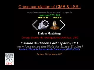
Cross-correlation of CMB & LSS :recentmeasurements, errors and prospectsastro-ph/0701393WMAP vs SDSSEnrique GaztañagaConsejo Superior de Investigaciones Cientificas, CSICInstituto de Ciencias del Espacio (ICE), www.ice.csic.es (Institute for Space Studies)Institut d'Estudis Espacials de Catalunya, (IEEC-CSIC)Santiago, 21-23rd March , 2007
Higher orders and ISW I- Perturbation theory and Higher order correlations II- CMB & LSS: ISW effect III- Error analysis in CMB-LSS cross-correlation
HOW DID WE GET HERE? • Two driving questions in Cosmology: • Background: Evolution of scale factor a(t). • + Friedman Eq. (Gravity?) • + matter-energy content • H2(z) = H20 [ M (1+z)3 + R (1+z)4 + K(1+z)2 + DE (1+z)3(1+w) ] • r(z) = dz/H(z) • Dark Matter and Dark Energy! • Structure Formation: • origin of structure (IC) • + gravitational instability • + matter-energy content • d’’ + H d’ - 3/2 Wm H2d = 0 • + galaxy formation (SFR) atoms Tiempo Energia
time Overdensed region Where does Structure in the Universe come From? How did galaxies/star/molecular clouds form? Small Initial overdensed seed background Collapsed region Perturbation theory: r = rb( 1 + d) => Dr = (r - rb ) = rbd • rb= M / V =>DM /M = d
Jeans Instability (linear regime) dL (x,t) = D(t) d0(x) EdS dL (x,t) = a(t) d0(x) • Another handle on Dark Energy (DE): • Friedman Eq. (Expansion history) can not separate gravity from DE • Growth of structure could: models with equal expansion history yield difference D(z) (EG & Lobo 2001), astro-ph/0303526 & 0307034) • how do you measure D(z) from observations? EdS Open z = 9 z = 0 (now) L a = 1/(1+z) a = 0.01 a = 0.1 a = 1 (now) a = 10
Argue that the linear growth equation: Has the following solutions: Problem I (2) Show that:
Spherical collapse model: In this case we can solve fully the non-linear evolution: results In a strongly non-linear collapse Critical density dc = 1.68 • Another handle on DE: • Models with equal expansion history yield difference D(z) and difference dc(EG. & Lobo, astro-ph/0303526 & 0307034)
Weakly non-linear Perturbations: Solved problem!?RPT (Crocce & Sccocimarro 2006) EdS vertices angular average d = dL + n2 dL2 + ... Leading order contribution in d corresponds to the spherical collapse.
Observations require an statistical approach: Evolution of (rms) variancex2= < d2>instead ofd Or power spectrumP(k)= < d2(k)> => x2 = ∫ dk P(k) k2 W(k) dk IC problem: Linear Theory d = a d0 x2 = < d2> = D2 < d02> Normalization s82º < d2(R=8)> To find D(z) -> Compare rms at two times or find evolution invariants Initial Gaussian distribution of density fluctuations: xp (V) = < dP>=0 for allp ≠2 Perturbations due to gravity generate non-Gaussian statistics xp -> x3 = S3x22with S3(m)= 34/7 (time & Cosmo invariant)
Predictions of Inflation Flat universe scale invariance IC: n~1 + CDM transfer funcion: P(k) = kn T(k) => Gaussian IC
Local spectral index P(k) ~ kn (initial spectrum + transfer function) x2[r]=∫ dk P(k) k2 W(k) dk ~ r-(n+3) n ~ -2 => x2 [r] ~ r -1(1D fractal ) equal power on all scales(Wm~0.2) n ~ -1 => x2 [r] ~ r -2(2D fractal ) less power on large scales(Wm~1.0) n ~ -2 CMB Superclusters Clusters Galaxies n ~ 1 Wm n ~ -1 Horizon @ Equality s8 SCDM n ~ -1 LCDM n ~ -2 Wm~1.0 Wm~0.2
Interest of Higher order PT or correlations: Gaussian IC? non-linearities: mode coupling non-linearities= non-gaussianities cosmic time invariants: do not depend much on cosmic history (cosmological parameters) bias: how light traces mass => measure mass
Weakly non-linear Perturbation Theory: Solved problem! vertices angular average d = dL + n2 dL2 + ... Leading order contribution in d corresponds to the spherical collapse.
Spherical collapse model: In this case we can solve fully the non-linear evolution: results In a strongly non-linear collapse Critical density dc = 1.68 • Another handle on DE: • Models with equal expansion history yield difference D(z) and difference dc(EG. & Lobo, astro-ph/0303526 & 0307034)
Weakly non-linear Perturbation Theory (Spherical average) d = dL + n2 dL2 + ... d3 = dL3 + 3 n2 dL4 + ... Gaussian Initial conditions < dL3 > = a3 <d03>= 0 < d3 > = < dL3 > + 3 n2 < dL4 > + ... < dL4 > = < dL 2 >2 < d3 > = 3 n2 < dL2 >2 + ... S3º< d3 > / < d2 >2 = 3 n2 =34 / 7 gravity? High order statistics -> vertices of non-linear growth!
Test in N-body simulations 3-pt funct N3 = (106)3 !!
Weakly non-linear Perturbation Theory Gaussian Initial conditions: connected correlations are zero, except 2-pt=> All correlations are built from 2-pt! Tree level= dominant = Tree level: F2 F3 Loops(higher order corrections): F2 F3 =
Weakly non-linear Perturbation Theory Tree level P(k) ~ kn 3 1 r23 a=q r12 2
Depends on local spectral index P(k) ~ kn (not on Wm) x2[r]=∫ dk P(k) k2 W(k) dk ~ r-(n+3) n ~ -2 => x2 [r] ~ r -1 (1D fractal ) equal power on all scales (Wm~0.2) n ~ -1 => x2 [r] ~ r -2 (2D fractal ) less power on large scales (Wm~1.0) n ~ -2 n ~ -2 n ~ -1 n ~ -1 n ~ -2 n ~ -1
Where does Structure in the Universe come From? How did galaxies/star/molecular clouds form? time Overdensed region Initial overdensed seed background Collapsed region IC + Gravity+ Chemistry = Star/Galaxy (tracer of mass?) dust H2 STARS D.Hughes
Bias: lets take a very simple model. rare peaks in a Gaussian field (Kaiser 1984, BBKS) Linear bias “b”:d(peak) = b d(mass) with b= n/s (SC:n=dc/s -> x2 (peak) = b2x2 (m) Threshold n
Biasing: does light trace mass? On large scales 2-pt Statistics is linear Gravity gbm Bias m = L D0 Gravity vs Galaxy formation gbm= b D0
Biasing: does light trace mass? Local approximation gF[m] gbm bm Lis Gaussian m is not mLL gbm= bL g b3m3 3 bb2 m4 g bbbg Gravity vs Galaxy formation c 2 b/ b c 3 b3/ b
Bias:rare peaks in a Gaussian field (Kaiser 1984. BBKS) Linear bias “b”:d(peak) = b d(mass) with b= n/s (for SCn=dc/s) -> x2 (peak) = b2x2 (m) Non-linear bias:-> b2= b2 ( bk= bk )-> Bias S3 = 3 S4 = 16 (Sk = kk-2) -> Close to DM!! Gravity S3 = 34/7-(n+3) ~ 3 S4 ~ 20 Threshold n How to separate one from the other?
How to separate Bias from Gravity? QG= (Qm+C)/B B<1 C Using scale or shape (configurational) dependence of 3-pt function: Fry & EG 1993; EG & Frieman 1994; Frieman & EG 1994; Fry 1994; Scoccimarro 1998; Verde etal 2001 B>1 CGF model: Bower etal 1993
Comparison with 2dfGRS • - Gravity @ work (astro-ph/0501637 & astro-ph/0506249) • -3pt correlation can be used to understand biasing: this is independent of normalization or cosmological parameters • 1st mesurement of galaxy bias (c2 and b) with 3pt function (away from b=1 and c2=0, Verde etal 2001) • b1= 0.95 0.12 b2 = -0.3 0.1 ( -0.4 <c2< -0.2) • Work in progress (by galaxy type and color) • measure of normalization: 0.8 < s8 < 1.0 • => Future applications? Gravity vs Galaxy formation
Bias & Higher: conclusion Local approximation works on larrge scales gF[m] For P(k) or 2-pt statistics: Linear theory works on scales > 10 Mpc But amplitude (b1) is unknown: degeneracy between D(z) or sigma8 and b1! For 3-pt statistics: Need higher bias coeffcients (b1, b2, b3…) But can define invariables (S3, Q3) that do not Depend on D(z). Can separate b1 from b2! => Need to find b1, b2, b3….
Higher orders and ISW I- Perturbation theory and Higher order correlations II- CMB & LSS: ISW effect III- Error analysis in CMB-LSS cross-correlation
Observations require an statistical approach: Evolution of (rms) variancex2= < d2>instead ofd IC problem: Linear Theory d = a d0 => x2 = < d2> = D2 < d02> Normalization s82º < d2(R=8)> To find D(z) -> Compare rms at two times or find evolution invariants
Perturbation theory: r = rb( 1 + d) => Dr = (r - rb ) = rbd • rb= M / V =>DM /M = d • With : d’’ + H d’ - 3/2 Wm H2d = 0in EdS linear theory: d = a d0 Gravitation potential: F = - G M /R =>DF = G DM / R = GM/R d in EdS linear theory: d = a d0=>DF = GM (d/ R) = GM (d0/ R0) !! Df is constant even when fluctuations grow linearly! We can mesure Df today an at CMB: should be the same! Where does Structure in the Universe come From?
PRIMARY CMB ANISOTROPIES Sachs-Wolfe (ApJ, 1967) DT/T(n) = [F (n) ]if Temp. F. = diff in N.Potential (SW) Ff Fi DT/T=(SW)= DF /c2 DF= GM (d/ R) /c2 CMB & LSS
Calculate the rms temperature fluctuation in the CMB due to the Sachs-Wolfe effect as a function sigma_8 (the linear rms density fluctuations on a sphere of radius 8 Mpc/h) and the value of Omega_m (fraction of matter over the critical density). Does the result depend on the cosmological constant (ie Omega_Lambda)? Problem II Ff Fi
PRIMARY & SECONDARY CMB ANISOTROPIES Sachs-Wolfe (ApJ, 1967) DT/T(n) = [ 1/4 dg (n) + v.n + F (n) ]if Temp. F. = Photon-baryon fluid AP + Doppler + N.Potential (SW) SZ- Inverse Compton Scattering -> Polarization Ff Fi + Integrated Sachs-Wolfe (ISW)+ lensing + Rees-Sciama + SZ 2 ∫if dtdF/dt(n) In EdS (linear regime) D(z) = a , and therfore dF/dt = 0 Not in L dominated universe !
CMB Noise Primary CMB signal becomes a contaminant when looking for secondary (ISW, SZ, lensing) signal. The solution is to go for bigger area. But we are limited by having a single sky. Noise! Signal Crittenden ISW map, z< 4 Early map, z~1000
Crittenden & Turok (PRL, 1995) Cross-correlation idea Both DT and d(g) are proportional to local mass fluctuations d(m)
(1) Assuming that galaxies trace the mass, demostrate that in the linear regime and for small angles (~<10 deg), the angular galaxy-galaxy correlation and the galaxy-temperature correlation (induced by ISW effect) are: Problem III sight (2) How does the above expressions change with linear bias?
ISW in equations... Limber approximation
APM APM 5.0 deg FWHM 0.7 deg FWHM WMAPAPM WMAPAPM WMAP WMAP 5.0 deg FWHM 0.7 deg FWHM
Possible ISW contaminants: • Primary CMB (noise) • Extincion/Absorption (of dust) in our galaxy • (CMB and LSS contaminants) • -Dust emission in galaxies/clusters • SZ effect • RS effect • CMB lensing by LSS structures • Magnification bias • … ?