An Introduction to Metaheuristics
1.33k likes | 2.19k Vues
An Introduction to Metaheuristics. Chun-Wei Tsai Electrical Engineering, National Cheng Kung University. Outline. Optimization Problem and Metaheuristics Metaheuristic Algorithms Hill Climbing (HC) Simulated Annealing (SA) Tabu Search (TS) Genetic Algorithm (GA)

An Introduction to Metaheuristics
E N D
Presentation Transcript
An Introduction to Metaheuristics Chun-Wei Tsai Electrical Engineering,National Cheng Kung University
Outline • Optimization Problem and Metaheuristics • Metaheuristic Algorithms • Hill Climbing (HC) • Simulated Annealing (SA) • Tabu Search (TS) • Genetic Algorithm (GA) • Ant Colony Optimization (ACO) • Particle Swarm Optimization (PSO) • Performance Consideration • Conclusion and Discussion
Optimization Problem • The optimization problems • continuous • discrete • The combinatorial optimization problem (COP) is a kind of the discrete optimization problems • Most of the COPs are NP-hard
D1 D1 D3 D3 D2 D2 D4 D4 1 2 3 4 1 2 3 4 1 2 3 4 1 2 3 4 1 2 3 4 1 2 3 4 1 2 3 4 1 2 3 4 s2 solution 3 2 3 2 The problem definition of COP • The combinatorial optimization problem P = (S, f) can be defined as: where opt is either min or max, x = {x1, x2, . . . , xn} is a set of variables, D1,D2, . . . ,Dn are the variable domains, f is an objective function to be optimized, and f : D1×D2×· · ·×DnR+. In addition, S = {s | s ∈ D1×D2×· · ·×Dn} is the search space. Then, to solve P, one has to find a solution s ∈ S with optimal objective function value. s1 solution 4 2 3 1
Combinatorial Optimization Problem and Metaheuristics (1/3) • Complex Problems • NP-complete problem (Time) • No optimum solution can be found in a reasonable time with limited computing resources. • E.g., Traveling Salesman Problem • Large scale problem (Space) • In general, this kind of problem cannot be handled efficiently with limited memory space. • E.g., Data Clustering Problem, astronomy, MRI
Combinatorial Optimization Problem and Metaheuristics (2/3) • Traveling Salesman Problem (n!) • Shortest Routing Path Path 1: Path 2:
opt Combinatorial Optimization Problem and Metaheuristics (3/3) • Metaheuristics • It works by guessing the right directions for finding the true or near optimal solution of complex problems so that the space searched, and thus the time required, can be significantly reduced.
The Concept of Metaheuristic Algorithms • The word “meta” means higher level while the word “heuristics” means to find. (Glover, 1986) • The operators of metaheuristics • Transition: play the role of searching the solutions (exploration and exploitation). • Evaluation: evaluate the objective function value of the problem in question. • Determination: play the role of deciding the search directions.
Transition Evaluation Determination Transition Evaluation Determination An example-Bulls and cows • Check all candidate solutions • Guess Feedback Deduction • Secret number: 9305 • Opponent's try: 1234 • 0A1B • 1234 • Opponent's try: 5678 • 0A1B • 5678 • number 0 and 9 must be the secret number from wiki
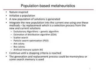
Classification of Metaheuristics (1/2) • The most important way to classify metaheuristics • population-based vs. single-solution-based (Blum and Roli, 2003) • The single-solution-based algorithms work on a single solution, thus the name • Hill Climbing • Simulated Annealing • Tabu Search • The population-based algorithms work on a population of solutions, thus the name • Genetic Algorithm • Ant Colony Optimization • Particle Swarm Optimization
Classification of Metaheuristics (2/2) • Single-solution-based • Hill Climbing • Simulated Annealing • Tabu Search • Population-based • Genetic Algorithm • Swarm Intelligence • Ant Colony Optimization • Particle Swarm Optimization
Hill Climbing (1/2) • greedy algorithm • based on heuristic adaptation of the objective function to explore a better landscape begin t 0 Randomlycreatea string vc Repeat evaluatevc selectm new strings from the neighborhood of vc Let vn be the best of the m new strings If f(vc) < f(vn) then vc vn t t+1 Untilt N end
Hill Climbing (2/2) Global optimum Local optimum Starting point Starting point search space
Simulated Annealing (1/3) • Metropolis et al., 1953 • From the annealing process found in thethermodynamics and metallurgy • To avoid the local optimum, SA allows worse moves with a controlled probability---temperature • The temperature will become lower and lower due to the convergence condition
Simulated Annealing (2/3) begin t 0 Randomlycreatea string vc Repeat evaluatevc select 3 new strings from the neighborhood of vc Let vn be the best of the 3 new strings If f(vc) < f(vn) then vc vn Else if (T > random()) then vc vn UpdateT according to annealing schedule t t+1 Untilt N end vc = 01110 f = 01110 = 3 n1 = 00110, n2 = 11110, n3 = 01100 vn = 11110 vc = vn= 11110
Simulated Annealing (3/3) Global optimum Local optimum Local optimum Starting point Starting point search space
Tabu Search (1/3) • Fred W. Glover, 1989 • To avoid falling into the local optima and searching the same solutions, the solutions recently visited are saved in a list, called the tabu list (a short-term memory the size of which is a parameter). • Moreover, when a new solution is generated, it will be inserted into the tabu list and will stay in the tabu list until it is replaced by a new solution in a first-in-first-out manner. • http://spot.colorado.edu/~glover/
Tabu Search (2/3) begin t 0 Randomlycreatea string vc Repeat evaluatevc select 3 new strings from the neighborhood of vc and not in the tabu list Let vn be the bestof the 3 new strings If f(vc) < f(vn) then vc vn Updatetabu list TL t t+1 Untilt N end
Tabu Search (3/3) Global optimum Local optimum Local optimum Starting point search space
Genetic Algorithm (1/5) • John H. Holland, 1975 • Indeed, the genetic algorithm is one of the most important population-based algorithms. • Schema Theorem • short, low-order, above-average schemata receive exponentially increasing trials in subsequent generations of a genetic algorithms. • David E. Goldberg • http://www.illigal.uiuc.edu/web/technical-reports/
Genetic Algorithm (4/5) • Initialization operators • Selection operators • Evaluate the fitness function (or the objective function) • Determinate the search direction • Reproduction operators • Crossover operators • Recombine the solutions to generate new candidate solutions • Mutation operators • To avoid the local optima
Genetic Algorithm (5/5) p1 = 01110, p2 = 01110 p3 = 11100, p4 = 00010 begin t0 initializePt evaluatePt while (not terminated) do begin t t+1 selectPt from Pt-1 crossover and mutationPt evaluatePt end end f1 = 01110 = 3, f2 = 01110 = 3 f3 = 11100 = 3, f4 = 00010 = 1 s1 = 01110 = 0.3, s2 = 01110 = 0.3 s3 = 11100 = 0.3, s4 = 00010 = 0.1 s4 = 11100 = 0.3 p1 = 011 10, p2 = 01 110 p3 = 111 00, p4 = 11 100 c1 = 011 00, c2 = 01 100 c3 = 111 10, c4 = 11 110 c1 = 01101, c2 = 01110 c3 = 11010, c4 = 11111 c1 = 01100, c2 = 01100 c3 = 11110, c4 = 11110 24
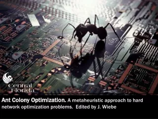
Ant Colony Optimization (1/5) • Marco Dorigo, 1992 • Ant colony optimization (ACO) is another well-known population-based metaheuristic originated from an observation of the behavior of ants by Dorigo • The ants are able to find out the shortest path from a food source to the nest by exploiting pheromone information • http://iridia.ulb.ac.be/~mdorigo/HomePageDorigo/
Ant Colony Optimization (2/5) food food nest nest
Ant Colony Optimization (3/5) Create the initial weights of each path While the termination criterion is not met Create the ant population s = {s1, s2, . . . , sn} Each ant si moves one step to the next city according the pheromone rule Update the pheromone End
Ant Colony Optimization (4/5) • Solution construction • for choosing the next sub-solution is defined as follows: where is the set of feasible (or candiate) sub-solutions that can be the next sub-solution of i; is the pheromone value between the sub-solutions i and j; and is a heuristic value which is also called the heuristic information.
Ant Colony Optimization (5/5) • Pheromone Update is employed for updating the pheromone values on each edge e(i, j), which is defined as follows: where is the number of ants; represents either the length of the tour created by ant k.
Particle Swarm Optimization (1/4) • James Kennedy and Russ Eberhart, 1995 • The particle swarm optimization originates from an observation of the social behavior by Kennedy and Eberhart • global best, local best, and trajectory • http://clerc.maurice.free.fr/pso/
Particle Swarm Optimization (2/4) • IPSO, http://appshopper.com/education/pso • http://abelhas.luaforge.net/
Particle Swarm Optimization (3/4) Create the initial population (particle positions) s = {s1, s2, . . . , sn} and particle velocities v = {v1, v2, . . . , vn} While the termination criterion is not met Evaluate the fitness values fi of each particle si For each particle Update the particle position and velocity IF (fi < f’i ) Update the local bestf’i = fi IF (fi < fg ) Update the global bestfg = fi End global best New motion trajectory, current motion local best, personal best
Particle Swarm Optimization (4/4) particle’s position and velocity update equations : velocity Vik+1 = wVik +c1 r1 (pbi-sik) + c2 r2(gb-sik) where vik: velocity of particle i at iteration k, w, c1,c2: weighting factor, r1, r2: uniformly distributed random number between 0 and 1, sik: current position of agent i at iteration k, pbi: pbest of particle i, gb: gbest of the group. position Xik+1 = Xik + Vik+1 Larger w global search ability Smaller w local search ability
Performance Consideration • Enhancing the Quality of the End Result • How to balance the Intensification and Diversification • Initialization Method • Hybrid Method • Operator Enhancement • Reducing the Running Time • Parallel Computing • Hybrid Metaheuristics • Redesigning the procedure of Metaheuristics
Large Scale Problem • Methods for solving large scale problems (Xu and Wunsch, 2008) • random sampling • data condensation • density-based approaches • grid-based approaches • divide and conquer • Incremental learning
opt opt How to balance the Intensification and Diversification • Intensification • Local Search, 2-opt, n-opt • Diversification • Keeping Diversity • Fitness Sharing • Increase the number of individuals • More computing resource • Re-create • Too much intensification local optimum • Too much diversification random search Intensification Diversification
Reducing the Running Time • Parallel computing • This method generally does not reduce the overall computation time. • master-slave model, fine-grained model (cellular model) and coarse-grained model (island model) [Cant´u-Paz, 1998; Cant´u-Paz and Goldberg, 2000] Population Sub-Population Island 2 Sub-Population Island 1 Migration procedure Sub-Population Island 3 Sub-Population Island 4
Multiple-Search Genetic Algorithm (1/3) The evolutionary process of MSGA.
TSP problem pcb442 Multiple-Search Genetic Algorithm (2/3) • Multiple Search Genetic Algorithm (MSGA) vs. Learnable Evolution Model (LEM) Tsai’s MSGA Michalski’s LEM
Multiple-Search Genetic Algorithm (3/3) • It may face the premature convergence problem because diversity of metaheuristics may decrease too quickly. • Each iteration may take more computation time than that of the original algorithm.
Pattern Reduction Algorithm • Concept • Assumptions and Limitations • The Proposed Algorithm • Detection • Compression • Removal
Concept (1/4) Our observation shows that a lot of computations of most, if not all, of the metaheuristic algorithms during their convergence process are redundant. (Data courtesy of Su and Chang) 43
C1 C1 C1 C1 1 0 1 0 1 1 0 0 1 1 0 0 0 1 0 1 1 1 1 1 1 1 1 1 0 0 0 0 0 0 0 0 C2 C2 C2 C2 C1 0 0 g =2, s =2 C2 1 1 . . . C1 0 0 Metaheuristics + Pattern Reduction g =n, s =2 C2 1 1 Concept (4/4) g=1, s =4 g =1, s =4 g=2, s =4 . . . g =n, s =4 Metaheuristics
Assumptions and Limitations Assumptions Some of the sub-solutions at certain point in the evolution process will eventually end up being part of the final solution (Schema Theory, Holland 1975) Pattern Reduction (PR) is able to detect these sub-solutions as early as possible during the evolution process of metaheuristics. Limitations The proposed algorithm requires that the sub-solutions be integer or binary encoded (i.e., combinatorial optimization problem). 47
The Proposed Algorithm Create the initial solutions P = {p1, p2, . . . , pn} While termination criterion is not met Apply the transition, evaluation, and determination operators of the metaheuristics in question to P /* Begin PR */ Detect the sub−solutions R = {r1, r2, . . . , rm} that have a high probability not to be changed Compress the sub−solutions in R into a single pattern, say, c Remove the sub−solutions in R from P; that is, P = P \ R P = P∪ {c} /* End PR */ End 49
Detection Time-Oriented Detect patterns not changed in a certain number of iterations aka static patterns Space-Oriented Detect sub-solutions that are common at certain loci Problem-Specific E.g., for the k-means, we are assuming that patterns near a centroid are unlikely to be reassigned to another cluster. T1: 1352476 T2: 7352614 T3: 7352416 … Tn: 7 C1416 T1 P1: 1352476 P2: 7352614 … Tn P1: 1 C1476 P2: 7C1614 50